In this article, we will go through how to built a multimodal LLM named Jñāna (sanskrit word for knowledge). You can try out the huggingface app Jñāna to see how it works. For video demo, go to the demo section below and for github code, go to the code section. This article mainly deals with 3 sections – Stage 1 training, Stage 2 training and building the app. Let us get started.

Table of contents

Introduction

Demo

Stage 1: Training the projection models

Stage 2 : Fine tuning the projection models and phi2

Stage 3 : Integrating audio and building Jñāna huggingface spaces app

Budget

Code

Credits

Contact Me

Introduction

Back to Top

Jñāna-Phi2-Multimodal-Conversation-Agent is a gradio app hosted on huggingface spaces. Jñāna is capable of accepting inputs in the form of image/audio/text or a combination of any of these 3 and returns output in the text format. Jñāna uses microsoft/phi2 LLM model that was trained based on Llava 1.0 and Llava 1.5 papers. Qlora PEFT strategy was used for fine-tuning phi2.

What is a multimodal LLM ? Traditional language models generally accepts text input alone and generates text based on the same. Whereas multimodal LLMs are capable of handling wide variety of input formats like image, audio, text and video. They are also capable of generating outputs in different formats like image, audio, text and video. A super multi-modal LLM will look like below:

In this article, we will be dealing only with image, audio, text inputs and will get text response as output. Let us delve into the training strategy and other details in below sections.

Demo

Back to Top

Below is an image inferred by Jnana accepting all 3 forms of input – image, audio and text. Audio query was “Please explain this image“. Also given below is youtube video link where you can find more demos for various combination of inputs: Jnana Youtube demo

Stage 1 : Training the projection models

Back to Top

Our objective here is to build a multimodal LLM. Multimodal means LLM should be capable to accept inputs in forms additional to usual text format. In our case, we are attempting to equip LLM to accept image and audio inputs apart from the text. We will use microsoft/phi2 as our LLM here. But phi2 is a textual LLM which means it accepts text tokens only as input. It doesn’t have innate capabilities to accept image or audio as input. So we have to convert image and audio to a format that phi2 can accept and understand. In stage-1, we will deal with converting image to an embedding format that phi2 can accept and process. Let us first understand the dataset and dataloading part required for stage-1 training.

Stage 1 : Dataset and dataloading

Back to Top

We will be using the images from instruct150k dataset and their corresponding captions from coco dataset. Instruct150k has 81479 images in it. All these images belong to the coco-train-2017-dataset. We will download the captions corresponding to these images from coco using !wget http://images.cocodataset.org/annotations/annotations_trainval2017.zip

We will then create a custom dataset that uses dynamic padding based on these images and captions. Code for the same is as below

class ClipEmbeddingDataset(Dataset):
    def __init__(self, image_names, caption_dict, tokenizer):
        self.data = image_names
        self.caption_dict = caption_dict
        self.tokenizer = tokenizer
        self.data_collator = DataCollatorWithPadding(tokenizer=self.tokenizer)

    def __len__(self):
        return len(self.data)

    def __getitem__(self, idx):

        return {
            'image_names': self.data[idx],
            'idx': idx
        }

    def tokenize_function(self, caption):
        return self.tokenizer(caption, truncation=True)

    def collate_fn(self, batch):
        image_names = [item['image_names'] for item in batch]
        captions = [self.caption_dict[image_name] for image_name in image_names]
        tokenized_caption_samples = []
        for caption in captions:
            tokenized_caption_dict = self.tokenize_function(caption)
            tokenized_caption_samples.append(tokenized_caption_dict)
        collated_captions = self.data_collator(tokenized_caption_samples)
        caption_tokens = collated_captions['input_ids']
        caption_attn_mask = collated_captions['attention_mask']

        return {
            'image_names': image_names,
            'captions': captions,
            'caption_tokens': caption_tokens,
            'caption_attn_mask': caption_attn_mask
        }

dataset = ClipEmbeddingDataset(image_names_lst, instruct150k_caption_data, tokenizer)

batch_size = 2
dataloader = DataLoader(dataset, batch_size=batch_size, collate_fn=dataset.collate_fn, shuffle=True)

In the code, dataset is created using below components:

• instruct150k_caption_data : This is a python dictionary that comprises of records in below format. Here each image correponding to instruct150k image is appended with strings _0, _1, _2, _3, _4 corresponding to their 5 coco captions. Thus, this will have 81479 * 5 records in it. But, we will use only 81479 out of it (first caption only)

{'000000318556.jpg_0': 'A very clean and well decorated empty bathroom',
 '000000318556.jpg_1': 'A blue and white bathroom with butterfly themed wall tiles.',
 '000000318556.jpg_2': 'A bathroom with a border of butterflies and blue paint on the walls above it.',
 '000000318556.jpg_3': 'An angled view of a beautifully decorated bathroom.',
 '000000318556.jpg_4': 'A clock that blends in with the wall hangs in a bathroom. ',
 '000000116100.jpg_0': 'A panoramic view of a kitchen and all of its appliances.',
 '000000116100.jpg_1': 'A panoramic photo of a kitchen and dining room',
 '000000116100.jpg_2': 'A wide angle view of the kitchen work area',
 '000000116100.jpg_3': 'multiple photos of a brown and white kitchen. ',
 '000000116100.jpg_4': 'A kitchen that has a checkered patterned floor and white cabinets.',
 ......
 '000000379340.jpg_4': 'A street sign modified to read stop bush.'}

• image_names_lst : This is a python list having the image names corresponding to the first caption alone i.e. ['000000318556.jpg_0', '000000116100.jpg_0', '000000379340.jpg_0',….,'000000134754.jpg_0']. This will have 81479 records in it.

• tokenizer : We will be using microsoft/phi2 tokenizer as below. We will also resize the token embeddings of phi2 model based on len(tokenizer). phi2 output embedding size is 51200 whereas length of our tokenizer here is 50295, hence resizing is done to avoid mismatch during training.

model_name = "microsoft/phi-2"
phi2_model = AutoModelForCausalLM.from_pretrained(model_name, trust_remote_code=True).to(device)

tokenizer = AutoTokenizer.from_pretrained(model_name, trust_remote_code=True, use_fast=False)
print(f'len(tokenizer 1: {len(tokenizer)}')

tokenizer.pad_token = tokenizer.eos_token
bos_token_id = tokenizer.bos_token_id
pad_token_id = tokenizer.bos_token_id
eos_token_id = tokenizer.bos_token_id
eoi_string = 'caption image:'
eoi_tokens = tokenizer.encode(eoi_string)
print(f'eoi_tokens : {eoi_tokens}')
print(bos_token_id, pad_token_id, eos_token_id)
print(tokenizer.decode([50256, 50256, 50256]))
print('eoi tokens decoded:', tokenizer.decode(eoi_tokens))
print(len(tokenizer)) # 50295

phi2_model.resize_token_embeddings(len(tokenizer))

• self.data_collator = DataCollatorWithPadding(tokenizer=self.tokenizer) -> This helps in dynamic padding. Refer HF Data Collator for more details. We will come to know how it helps in dynamic padding once we inspect the code below.

Now, let us inspect each part of dataset code to understand its working.

    def __init__(self, image_names, caption_dict, tokenizer):
        self.data = image_names
        self.caption_dict = caption_dict
        self.tokenizer = tokenizer
        self.data_collator = DataCollatorWithPadding(tokenizer=self.tokenizer)

This is the init method of our ClipEmbeddingDataset class.

    def __len__(self):
        return len(self.data)

    def __getitem__(self, idx):

        return {
            'image_names': self.data[idx],
            'idx': idx
        }

This is __len__ and __getitem__ methods of our ClipEmbeddingDataset class. Please note that we are driving our data generation using self.data which is image_names_lst – python list having image names like ['000000318556.jpg_0', '000000116100.jpg_0']

    def tokenize_function(self, caption):
        return self.tokenizer(caption, truncation=True)

    def collate_fn(self, batch):
        image_names = [item['image_names'] for item in batch]
        captions = [self.caption_dict[image_name] for image_name in image_names]
        tokenized_caption_samples = []
        for caption in captions:
            tokenized_caption_dict = self.tokenize_function(caption)
            tokenized_caption_samples.append(tokenized_caption_dict)
        collated_captions = self.data_collator(tokenized_caption_samples)
        caption_tokens = collated_captions['input_ids']
        caption_attn_mask = collated_captions['attention_mask']

        return {
            'image_names': image_names,
            'captions': captions,
            'caption_tokens': caption_tokens,
            'caption_attn_mask': caption_attn_mask
        }

collate_fn is the main method of our dataset class. It accepts the batch that we get from __getitem__ method.

• It will collect image names in a list image_names = [item['image_names'] for item in batch]
• It will collect captions also in a list captions = [self.caption_dict[image_name] for image_name in image_names]

• Then it will tokenize each caption and write it to another list tokenized_caption_samples

        tokenized_caption_samples = []
        for caption in captions:
            tokenized_caption_dict = self.tokenize_function(caption)
            tokenized_caption_samples.append(tokenized_caption_dict)

• This list of captionized tokens is passed through data collator collated_captions = self.data_collator(tokenized_caption_samples)
• Here, data_collator will make the caption lengths uniform. Let us say we have 2 captions of token lengths 10 and 15 each. Then, the 15 token caption will be kept as such. The 10 token caption will be padded by 5 tokens so that it will also have 15 tokens. Thus, in a batch all the captions will match the size of the biggest caption present. An example shown as below. Here 1st token is padded by 1 token (50256) to match the length of longest caption – 13.

['One sheep running through the shrub brush of a field.', 'The view of a kitchen with a window that is opened slightly.']
torch.Size([2, 13]) 
tensor([[ 3198, 15900,  2491,   832,   262, 10157,   549, 14093,   286,   257,  2214,    13, 50256],
        [  464,  1570,   286,   257,  9592,   351,   257,  4324,   326,   318,  4721,  4622,    13]])

• collated_captions coming out from data collator will be a dictionary having 2 keys – ‘input_ids’ and ‘attention_mask’
• ‘input_ids’ will have the list of caption tokens
• ‘attention_mask’ will have the masks where tokens that need to be attended will have 1s whereas irrelevant tokens will hav 0s (padded tokens). We wont use this.
• We will capture input_ids & attention_mask as below

        caption_tokens = collated_captions['input_ids']
        caption_attn_mask = collated_captions['attention_mask']

• Finally we will return this as below

        return {
            'image_names': image_names,
            'captions': captions,
            'caption_tokens': caption_tokens,
            'caption_attn_mask': caption_attn_mask
        }

• Next we will create dataset as below

dataset = ClipEmbeddingDataset(image_names_lst, instruct150k_caption_data, tokenizer)

• Then we will create a dataloader that will be used for data generation while training

batch_size = 2
dataloader = DataLoader(dataset, batch_size=batch_size, collate_fn=dataset.collate_fn, shuffle=True)
print(len(dataset)) # 81479

• Sample records that will be coming out will look like below:

for idx, batch in enumerate(dataloader):
    image_names = batch['image_names']  # List of image names corresponding to each data slice
    captions = batch['captions']  # List of captions corresponding to each data slice
    caption_tokens = batch['caption_tokens']  # Shape: [batch_size, max_seq_len]
    caption_attn_mask = batch['caption_attn_mask']
    print(idx)
    print(image_names)
    print(captions)
    print(caption_tokens.shape, caption_tokens)
    print(caption_attn_mask.shape)
    print('---------')
    if idx > 0:
        break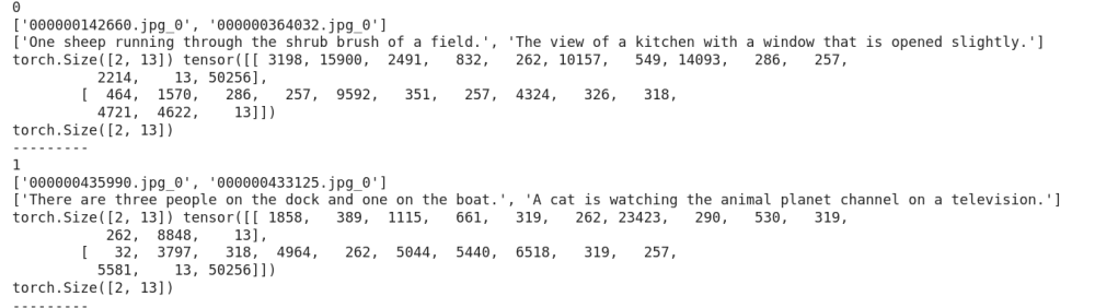

Now, let us look how training is done.

Stage 1 : Training

Back to Top

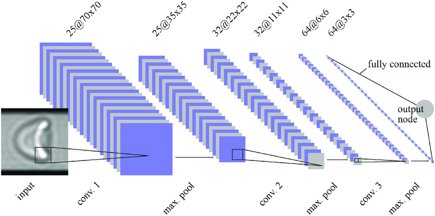
Below is a snap depicting the overall flow of stage-1 :

• We will pass the image to a CLIP model – openai/clip-vit-base-patch32. We will take the image embeddings from CLIP – one before projection layer whose shape is [50, 768]. As suggested in Llava1.0 paper we will discard the 1st layer that has CLS embeddings and retain [49, 768].
• We will pass this [49, 768] through a linear layer that will convert Clip embeddings to phi2 embedding dimensions i.e. from [49, 768] to [49, 2560]. We will then pass this [49, 2560] through projection model (Reference : Llava 1.5 Simple Res Block ). This projection model is responsible for making clip embeddings understandable to the phi2. In other words, projection model will capture the meaning of image and share it with phi2.
• phi2 used is pre-trained version from HF and in this stage we wont fine-tune phi2. Same goes for Clip as well i.e. phi2 and clip weights will remain frozen while projection linear layer and projection weights will get trained.
• Projection model will give us [49, 2560] as output. We will append an end-of-image token to this [49, 2560] to indicate that image embeddings ended. We used the text “caption image:” as end-of-image string. This EOI string was tokenized using microsoft/phi2 tokenizer that we created above.
• These EOI integer tokens were then passed through input-embed layer of pretrained phi2 model to get [4, 2560] where 2560 is the phi2 embedding dimension.Then, this [4, 2560] will be appended with the [49, 2560] that we got from projection model to get [53, 2560]. We will pass this [53, 2560] embeddings to phi2 forward method again & again until the caption length of image is matched as seen below. We will extract the last layers correpsonding to the caption and compare it with ground truth caption for loss calculation.
• Loss is backpropagated, projection linear layer and projection model weights updated and next batch picked-up. Loss used is cross_entropy loss.
• Training loop is as shown below:

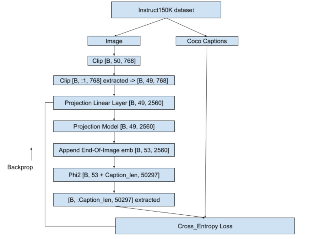
Training was done on ~30K images out of 81K on A100 (40GB VRAM gpu) and stopped when loss value dropped from 9.8783 to 1.1321. Teacher-forcing was used while training to help faster convergence and batch-size used was 2. This training consumed approximately 200 GPU compute units in google colab. Details of training can be seen in ‘Teacher forcing + Calling embeddings each time with EOI token as “caption image:” for 81K images’ section in the colab notebook ERA1_s29_stage1_experiment_v1.ipynb

Now with our projection model trained, let us move to stage 2 of training.

Stage 2 : Fine tuning the projection models and phi2

Back to Top

Pretrained phi2 is capable of only generating text. We have to fine-tune phi2 to engage in a conversation i.e when asked a query it should be able to answer it sensibly. In stage 1, we trained projection model which will now give us meaningful context about the image. In stage 2, we will fine-tune the phi2 so that it will become capable to handle a conversation. We will also fine-tune the projection linear layer and projection model so that they continue to learn about the images from the conversation data also. Let us first look into the dataset and dataloader part.

Stage 2 : Dataset and dataloader

Back to Top

Training was done on instruct150K dataset in stage 2 also. However, in stage-1 we trained instruct150k images against coco-captions, whereas here we will use the images with question/answer format present in instruct150k. This is because our training objective in stage-2 is to make phi2 capable for conversations.

• Instruct150k conversation were broken down into question-answer format and in total 3_56_752 records were there. This json format was sorted based on ascending order of answer length. Then, answer lengths upto 119 tokens that comprises 2_60_564 records were trained against T4 GPU (15 GB VRAM) in different batches. Different batch_sizes were choosen to avoid OOM issues as below:
  • Answer length 1 to 11 : 45557 records : bs = 10
  • Answer length 12 to 17: 53028 records : bs = 10
  • Answer length 18 to 23: 44613 records : bs = 9
  • Answer length 24 to 40: 52452 records : bs = 8
  • Answer length 41 to 59: 13482 records : bs = 6
  • Answer length 60 to 79: 21832 records : bs = 5
  • Answer length 80 to 99: 16162 records : bs = 4
  • Answer length 100 to 119: 28228 records : bs = 4

• Code for dataset is as below:

class ClipEmbeddingDataset(Dataset):
    def __init__(self, data, tokenizer):
        self.data = data
        self.tokenizer = tokenizer
        self.data_collator = DataCollatorWithPadding(tokenizer=self.tokenizer)

    def __len__(self):
        return len(self.data)

    def __getitem__(self, idx):

        return {
            'image_names': self.data[idx][-1]['image'],
            'idx': idx,
            'qn_text': self.data[idx][-1]['qn'],
            'ans_text': self.data[idx][-1]['ans']
        }

    def tokenize_function(self, caption):
        return self.tokenizer(caption, truncation=True)

    def collate_fn(self, batch):
        image_names = [item['image_names'] for item in batch]
        qns = [item['qn_text'] for item in batch]
        ans = [item['ans_text'] for item in batch]
        tokenized_qns_lst = []
        for qn in qns:
            tokenized_qns_dict = self.tokenize_function(qn)
            tokenized_qns_lst.append(tokenized_qns_dict)
        collated_qns = self.data_collator(tokenized_qns_lst)

        tokenized_ans_lst = []
        for an in ans:
            tokenized_ans_dict = self.tokenize_function(an)
            tokenized_ans_lst.append(tokenized_ans_dict)
        collated_ans = self.data_collator(tokenized_ans_lst)
        qn_tokens = collated_qns['input_ids']
        an_tokens = collated_ans['input_ids']

        return {
            'image_names': image_names,
            'qn': qn_tokens,
            'ans': an_tokens
        }

dataset = ClipEmbeddingDataset(stage_2_data_c100_119, tokenizer)

batch_size = 9
dataloader = DataLoader(dataset, batch_size=batch_size, collate_fn=dataset.collate_fn, shuffle=True)
print(len(dataset))

ClipEmbeddingDataset is created from python lists like stage_2_data_c100_119. Here c100_119 means answer lengths corresponding between 100 and 119 are considered. Similarly, if it was 80 to 99 then the name of that list will be stage_2_data_c80_99 and so on.

This python list (eg: stage_2_data_c100_119) contains a collection of lists. Each list corresponds to a single conversation. List will have two elements – first element is the answer length, second element is a dictionary. Dictionary will have following keys : 'image', 'qn', 'ans'. Here 'image' holds the image name. 'qn' holds the question related to the image and'ans' holds answer to that question. A sample record is as shown below:

'image' : '000000211217.jpg'
'qn' : 'What does the image suggest about the man's skill or experience with playing frisbee?'
'ans': 
'Note that while the image provides some clues about the man's potential abilities, it is not definitive proof of his expertise. It is, however, a representation of an individual enjoying and engaging in a physical activity that requires coordination and skill, showcasing the flexibility and versatility of the human body in motion'

Dataset creation is similar to stage-1. Here dynamic padding will be applied to both question and answer. For example, if biggest question length in the batch is 15, then all the shorter questions in the batch will be padded to 15. Same applies for answer too.

Stage 2 : Training

Back to Top

• While training, we will append the [53, 2560] that we get as output from projection model with the query embeddings and then generate the answer. This answer will be then compared with the ground truth answer.
• To stay within the memory constraints, phi2 will be downloaded in 4-bits and trained using peft-qlora strategy.Peft-qlora strategy will add adapter weights on top of the pretrained phi2 model which comes to be around just 3% of total weights trainable params: 94,371,840 || all params: 2,869,421,175 || trainable%: 3.28 which is light-weight and manageable
• Unlike stage 1, stage 2 was trained with a single model.forward() call to phi2 making it memory efficient. Let us understand the training flow using below image:

For an answer of 30 tokens and question of 20 tokens, training happens as below:

• Input <img emb [B, 49, 2560] > + <EOI [B, 4, 2560]> + <Qn [B, 20, 2560]> + <EOQ [B, 4, 2560]> + <Ans [B, 30, 2560]>
  • <EOI [B, 4, 2560]> -> EOI used is same as in stage-1 i.e. “caption image:”
  • <EOQ [B, 4, 2560]>-> EOQ i.e End Of Question used is “end of question:”

• Input shape will be [B, 107, 2560]
• Input goes to model.forward() and gets back logits of [B, 107, 50257]
• preds = Take final token of EOQ + last 30 tokens which will be [B, 76:, 50257]
• Add End-of-Sentence “<|endoftext|>” token to the answer target
• Compare preds with target for loss calculation

Loss calculation happens as below. Shown below is for a single batch but it can scale to any number of batches. Loss used is cross-entropy loss here as well.

• In this example, when last token of EOQ “:” is encountered, model is expected to predict first word of the answer which is “The“
• Similarly when “The” is seen, model should predict “color” and so on
• Finally when “.” is seen, model should predict “<|endoftext|>“
• As we can see, in the image above except for 3 tokens (circled in red), model got it correct

This training consumed approximately 110 GPU compute units in google colab. Training loss started at 3.634 at first batch and came down to 1.2028 at the final batch. Once training was done, fine-tuned phi2 qlora model was merged with publically available existing huggingface microsoft/phi2 model. This new model now available in HF as anilbhatt1/phi2-proj-offset-peft-model was used for inferencing in the Jñāna app.

Details of stage-2 training can be seen in the colab notebook ERA1_s29_stage2_experiment_v1.ipynb

Now, let us move to the audio-integration and inferencing part

Stage 3 : Integrating audio and building Jñāna huggingface spaces app

Back to Top

In stage 2, we equipped our model to accept an image and strike a conversation based on that image or textual query that we supply. However, our objective is to have our app capable of handling audio query as well. There are 2 ways to deal with audio:

1. Develop a projection model and train like we did in stage-1 and integrate it with phi2
2. Take an already available audio model, feed the audio to this model, get the text as output and feed this text as a query to multimodal LLM model

We will follow the latter approach i.e. using an existing audio model. We will use the whisperx model for handling the audio query. Below portion of code will accept the audio, convert it to text and tokenize it to feed to our stage-2 trained model.

        !pip install -q git+https://github.com/m-bain/whisperx.git
        import whisperx
        audio_model = whisperx.load_model("small", "cuda", compute_type="float16")
        audio_result = audio_model.transcribe(audio)
        audio_text = ''
        for seg in audio_result['segments']:
            audio_text += seg['text']
        audio_text = audio_text.strip()
        audio_tokens = tokenizer.encode(audio_text)

Then we will prepare the input_embed as below as applicable in below sequence:

image embed [49, 768] (if image present) + eoi [4, 768] + audio-qn embed (if audio present) + text-qn embed (if text present) + eoq [4, 768]

This input_embed is fed to model to generate output response text as below:

        max_len = 200
        output = self.phi2_model.generate(inputs_embeds=input_embed,
                                          max_new_tokens=max_len,
                                          return_dict_in_generate = True,
                                          bos_token_id=bos_token_id,
                                          pad_token_id=bos_token_id,
                                          eos_token_id=bos_token_id)

Details of inferencing tried in google colab can be found in ERA1_s29_Gradio_v1.ipynb

Budget

Back to Top

Overall it costed me ~ ₹4000 (around $50) to develop this LLM apart from my 3 weeks personal effort. Break-down of costs as follows:

• ~ $12 for 4 RTX 3090 GPUs to train phi2 from scratch on stage-0
• ~ $26 for A100 compute units to train proj model on stage-1
• ~ $12 for T4 compute units to fine-tune proj model and phi-2 on stage-2
• Inferencing was experimented in free colab T4 GPU

Code

Back to Top

• Github : https://github.com/anilbhatt1/Jnana_phi2_multimodal_llm

• Details of stage-1 training can be seen in ‘Teacher forcing + Calling embeddings each time with EOI token as “caption image:” for 81K images’ section in the colab notebook ERA1_s29_stage1_experiment_v1.ipynb

• Details of stage-2 training can be seen in the colab notebook ERA1_s29_stage2_experiment_v1.ipynb

• Details of inferencing tried in google colab can be found in ERA1_s29_Gradio_v1.ipynb

Credits

Back to Top

• Rohan Shravan, The School of A.I.
• whisperX for audio
• Llava 1.0 paper
• Llava github
• GPT LLM trainer
• HF PEFT training pytorch example

Contact Me

Back to Top

Connect me in linkedin at Anil Bhatt

Credits : The School Of AI

Github code for this post is here

Objective of this article:

1. Create a docker image for image classification with pytorch for cpu
2. Push this to docker hub – https://hub.docker.com/
3. Pull this image into another session & do inferencing running the docker cli command

You can use gitpod.io if there are space limitations in your machine. To use gitpod follow the below steps:

• You need to have a github repo as pre-requisite
• Then, go to https://www.gitpod.io/
• Click Try For Free and login with github as shown below

• Click on new workspace

• Select a github repository (here I selected EMLO2_S1_Docker)

• Give continue after confirming remaining options

• We can also see that there is enough space available (1.1 TB)

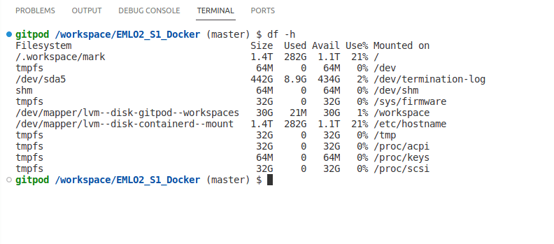
Now, let us get into docker image creation part

1. Create a docker image for image classification with pytorch for cpu

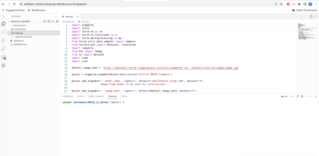
In this article, we are doing an image classification with pytorch. Let us get familiarized with the various files. You can get these files from the github link provided at the begining.

• main.py
  • This file does the inferencing logic.
  • It accepts a timm model (if you dont know timm, then refer Using Timm in HF and Timm Article by Chris Hughes)
  • It also accepts an image url or image path
  • It passes the image as input to the timm model and returns the classification result
• requirements.txt
  • This file has the requirements to be installed in docker
  • We are installing cpu versions of pytorch and torch-vision as GPU versions wiill cause docker image size to be huge
• Dockerfile
  • This file is used for installing the docker image
  • Entrypoint given is via entrypoint.sh
• entrypoint.sh
  • This will run python3 main.py “$@”
  • “$@” -> This indicates that pass whatever arguments supplied during docker run command to main.py

Next, build the docker image in local. Here we are building docker image named emlo2s1docker via the docker command as shown below

docker build -t emlo2s1docker .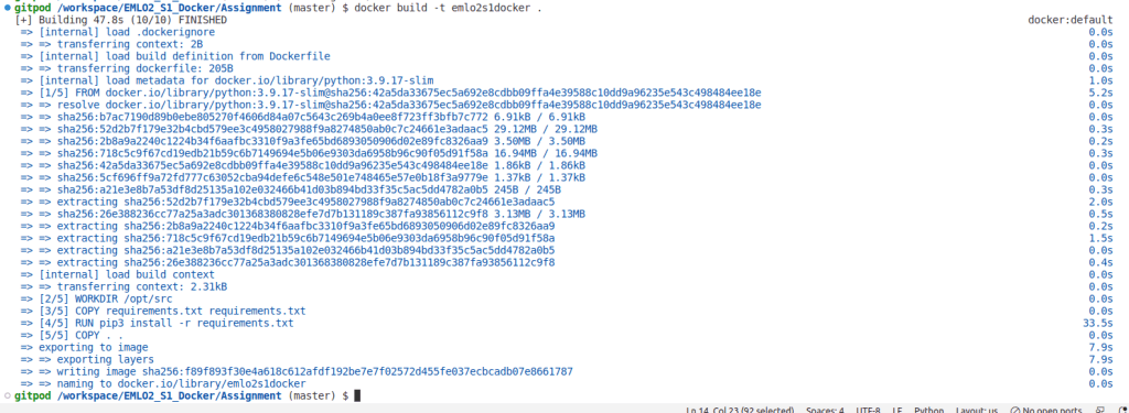

2. Push this to docker hub – https://hub.docker.com/

• Go to docker hub https://hub.docker.com/→ login with your credentials
• Create a public repository there (in this example emlo2s1docker)
  • It is better to keep repo name same as image name

• Next, login to docker in local using dockerhub user-id & password

• Tag the docker image as below using the docker command
  • Here we are tagging the emlo2s1docker image present in our local with anilbhatt1/emlo2s1docker repo that we created in docker hub above.

docker tag emlo2s1docker anilbhatt1/emlo2s1docker 

• Push the image to docker hub public repo

docker push anilbhatt1/emlo2s1docker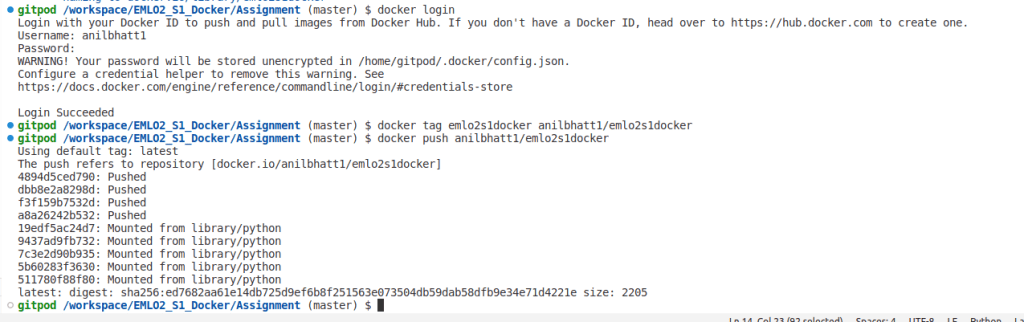

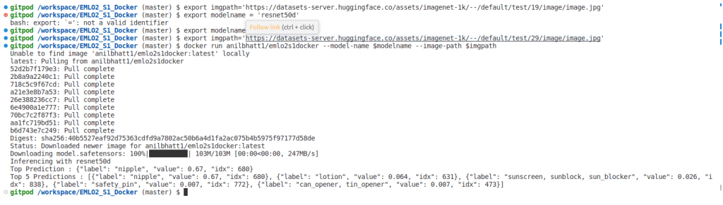
• If all went fine, we should see the image pushed to repo as shown below

3. Pull this image into another session & do inferencing

• Now, we can pull image anywhere in the world via below command

docker pull anilbhatt1/emlo2s1docker

• Now, let us run the docker image
  • We are exporting the image url to an env variable called imgpath
  • We are exporting the model name to an env variable called modelname
  • Then, we are running the docker image by passing these as arguments

export imgpath='https://datasets-server.huggingface.co/assets/imagenet-1k/--/default/test/19/image/image.jpg'
export modelname='resnet50d'
docker run anilbhatt1/emlo2s1docker --model-name $modelname --image-path $imgpath

• Image passed was a nipple

• As, we can see inferencing happened correctly as ‘nipple’ with resnet50d

YOLO – ‘You Only Look Once’ is state of art algorithm used for real-time object detection. Since its inception Yolo went through several revisions and latest version Yolo V5 was launched few weeks back. This article is not specific to any version but will give an overall idea how Yolo works. Aim of this article is to develop an intuition how Yolo detects an object which in turn will help understand the official Yolo papers and future revisions.

1. Let us start with Classification vs detection

Classification tells us the object classes present in image whereas detection gives us the location + class names. We call those rectangles that show the location of the object – Bounding Boxes (BB).

2. Predictions in object detection

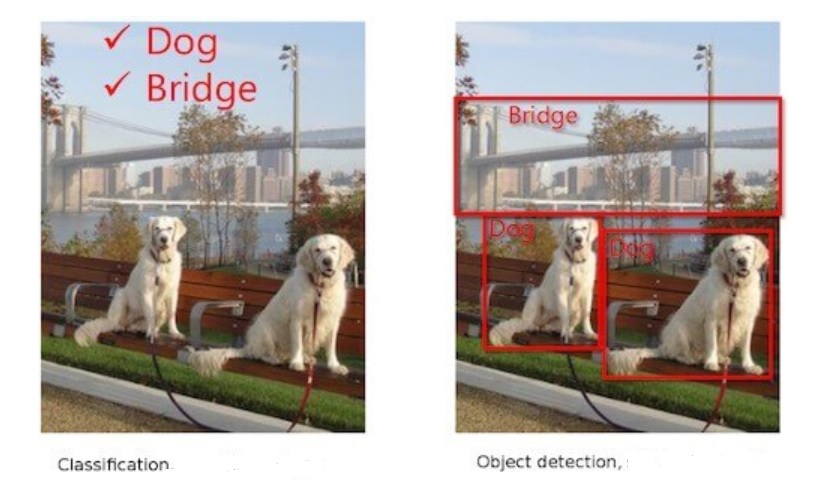
Object classification only has to tell us which object a particular image contains – dog, bridge etc. However, job of object detection is more tough. It has to predict the class as well as show the location. As shown below, algorithm should detect object/s and bound each of them – in this case person, bottle, laptop and chair.

For object classification, one hot vector prediction will be as follows for the above image:
Person – 0, One hot vector : [1,0,0,0]
Bottle – 1, One hot vector : [0,1,0,0]
Laptop – 2, One hot vector : [0,0,1,0]
Chair – 3, One hot vector : [0,0,0,1]

For object detection, prediction should include BB coordinates as well. Network needs to predict a minimum of 5 parameters – x, y (centroid coordinates of object), w, h (width & height of BB) and class. A network will predict accurately only if we train it properly. Hence for object detection network, training labels need to have following parameters – x, y (centroid coordinates of GT), w, h (width & height of GT BB) and class. We will see how Yolo predicts later in this article. * GT – Ground Truth

3. Quick recap – Object classification

Let us take a look at how object classification works via CNN.
– Convolutions are performed on original image.
– Image is broken into edges & gradients.
– Patterns are reconstructed from these edges & gradients.
– Then part of objects and eventually objects are reconstructed.
– If we convolve further, scenes are reconstructed.
Just before GAP layer, neurons will light up as below. ( Unlike below, size of final feature map may be smaller than the original image size depending on the network stride. eg: Image Size: 416, stride : 32, then final feature map size = 416/32 = 13)

Few pixels will be brighter than remaining pixels like the one that is bounded in above image. What this means is network found this particular feature strongly correlated with the class it is going to predict. For example, nose of dog could be the feature that network found unique for the dog class. These pixel/s are of great importance for Yolo.

4. Basic Idea – How Yolo Predicts ?

Initial epochs of Yolo network are trained only for classification. For subsequent epochs, both detection and classification are trained. During initial epochs network is just learning about the object it has to classify. Hence, it doesn’t make sense to ask the network to predict the BB at this point when it is not even certain about the object. As we have seen above, once network becomes adept at classification, some pixels will light-up more than others as we have seen above. Yolo will take the brightest pixel among these, find its centroid and put a bounding box around it. This is the basic idea how Yolo detects objects. Let us dive deeper to understand how this is done.

5. Objectness – How Yolo determines brightest pixel/s ?

Let us understand how Yolo identifies the brightest pixel/s so that network can focus only on those and ignore the rest. Yolo will break the image of size let us say 416×416 to a grid of fixed size say 13×13 (Why 13 x 13, we will see in section 10). As network trains in classification, it starts assigning a parameter called objectness score (OS) to all the cells.

Objectness means how much probability does a cell thinks it has an object inside it. Once OS is assigned, Yolo will filter the cells based on an objectness threshold. Let us say threshold is set at 0.8. Only those cells that have OS > threshold will be considered for further analysis. Yolo achieves this by assigning a parameter called Objectness number (1obj) to each cell. Those cells having OS above threshold will be assigned a value of 1 for 1obj. For all other cells Objectness number will be set to 0. Let us say in our 13×13 grid, only 2 cells qualified the OS threshold. Then only these 2 cells will be assigned 1obj value of 1 , remaining 167 cells will be assigned 1obj = 0. We will understand how 1obj helps to ignore below threshold cells once we examine the Yolo loss function.

Let us say 3 cells qualified. This could mean two things:
1) There were three objects as in fig-1 i.e. 2 dogs and a bridge. If so, we are good.
2) But what if image has only object. This means adjacent cells belonging to the same object passed the objectness threshold. In such a case, Yolo will choose the best cell out of these 3 based on a method called Non-Maximum Suppression(NMS) with the help of objectness score and IOU. More on these later.

6. Anchor Boxes in Yolo

Yolo network mainly has 2 tasks – classification and detection. As mentioned earlier, detection means detecting the location of centroid and BB width and height. Yolo uses concept of anchor boxes to bound the object. So, what are anchor boxes and why are they needed ? Each object is unique and will have its own size and shape. Box that can bound a bird may not be able to bound a car. So, bounding boxes will differ based on the object class as well as pose. Instead of creating a bounding box on the fly during training, Yolo uses fixed number of template boxes (3 or 5) that we call anchor boxes (priors – in official paper). How this fixed number is arrived ? We will see in Section 7.

Imagine packing your household items as part of shifting home. Creating a customized box for each item will end-up creating 100s of boxes. So pragmatically, we select few template boxes in which we will pack the things. Let us say your television set doesn’t fit to any of the templates. You found one of the templates slightly big but closely matching. You will use this template but fill the extra spaces with thermocol or clothes so that TV will stay tight. Similar concept is used in Yolo. In Yolo, we will use anchor boxes to bound the objects. These anchor boxes wont be perfect fit for the objects that Yolo detects. Hence as seen with TV set, Yolo will choose the best matching anchor box and scale it appropriately to bound the object. Yolo V2 uses 5 anchor boxes while Yolo V3 used 3 anchor boxes. In this article, we will stick on with 5 anchor boxes.

In order to scale the anchor boxes, we need some factor by which dimensions should be scaled. From where we get these scaling factors ? Answer – network will predict the factor by which anchor box height and width need to be scaled up/down. Based on these predicted factors, Yolo will scale the anchor boxes thus giving us bounding boxes.

7. How to select the best bounding box ?

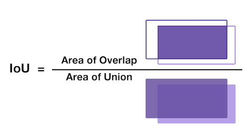
As decided in prior section, we will use 5 anchor boxes in this article. What this means is that for each cell, network will predict 5 boxes. Based on objectness number, objectness score and using NMS, network will filter down the number of cells to one cell per object. This cell will have 5 bounding boxes corresponding to the 5 anchor boxes we are using. But we need only 1 box to bound an object. How Yolo chooses 1 out of these 5 boxes ? This is where IOU comes into picture. As we have seen in section 2, training labels that we supply for Yolo will have ground truth for class, object centroid location & bounding box width and height. Based on these ground truth coordinates, we will get ground truth bounding box area. Yolo will predict centroid locations and scaling factors for each of 5 anchor boxes. Based on these, we will get predicted area for 5 bounding boxes. Yolo will choose the box with highest IOU.

What is IOU ? IOU means Intersection over union. It is a measure that gives how much area you have in common between prediction and ground truth. Higher the IOU, better the prediction. So out of 5 predicted boxes, Yolo will choose the box with highest IOU. Below image helps to understand IOU better.

Collision : Let us say one cell itself is having multiple object. Let us take the fig-2 and assume that bottle & laptop are in same cell. Yolo predicts 5 bounding boxes per cell. Let us see how bounding boxes are getting assigned to bottle & laptop in this case. Yolo uses a method called collision in such instances. This is how it happens.

• Yolo predicts the classes for the objects identified in the cell and objectness score.
• Yolo predicts the centroid & bb scale coordinates for the classes.
• Yolo calculates the area of scaled bounding boxes for each of the anchor boxes.
• Then it calculates IOU corresponding to each bounding box for each object.
• Anchor box that gets the best IOU will be selected & BB created out of that anchor box will be used forward.
• Let us name the 5 anchor boxes as A, B, C, D, E.
• Bottle is considered first. Anchors A, B, C, D, E share an IOU of 0.73, 0.57, 0.61, 0.52 and 0.45 respectively for bottle. Hence anchor A is assigned as it has highest IOU 0.73
• Next laptop is considered. Imagine laptop shares an IOU of 0.74, 0.68, 0.59, 0.53 and 0.47 with anchors A, B, C, D and E respectively.
• Now Yolo recognizes that laptop is better match for anchor A.
• Accordingly, it reassigns anchor A to laptop and assign Anchor C – the next best match (0.61) – to bottle.

8. How to decide the number of anchor boxes to be used ?

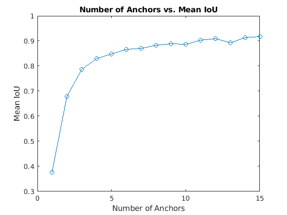
Anchor boxes are critical in determining the bounding boxes and thereby for Yolo object detection. So are we choosing the number of anchor boxes randomly ? No ! As part of pre-processing, we will pass the training data through a K-Means clustering and will choose a number that gives an optimal result between IOU and performance. Let us say we have 1 million unique objects in our dataset. We will get a mean IOU (Total IOU / No: of Images) of 1 if we choose 1 million BB. But this is not practical. Also beyond a certain point, IOU curve will flatten i.e. diminishing returns will start setting similar to what is shown below.
Hence Yolo researchers decided to settle on a number where algorithm can achieve good IOU without compromising performance (i.e. ability to detect on a real time basis). They tested Yolo on COCO and Imagenet datasets. Accordingly for Yolo V2 – 5 anchor boxes were used and in Yolo V5 – brought it down to 3 anchor boxes.

9. Yolo predictions

Based on what we understood so far, Yolo will predict class, objectness, centroid of object detected and bounding box scales. Let us try to visualize it.

• Image is broken down to S x S grid. In the above figure 13 x 13 cells.
• What we are seeing above with green steps is 1 such cell out of 169 cells.
• This cell will be having 5 anchor boxes (steps in figure).
• We are seeing expanded version on 1 such anchor box out of 5 anchor boxes.
• 1 anchor box will bound only 1 object. This anchor box will hold the objectness score of the object it detected (brown cell).
• Let us say we have 20 classes in our dataset. Prediction vector for the anchor box will have probability scores for these 20 classes (pink cells).
• Out of these 20, one that has highest score is the object that this specific anchor box detected (not shown in image).
• There will be 4 coordinates (yellow cells). First 2 coordinates belong to the centroid of the object detected.
• Next 2 coordinates belong to the bounding boxes (scaling factor).

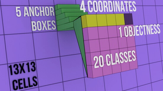
In the above image, each cell can have 5 anchor boxes, hence each cell can predict 5 different objects. Here, Yolo can predict a total of 169 * 5 = 845 objects out of entire 13×13 image grid . Each cell can have 5 anchor boxes each having 4 coordinates + 1 OS + 20 classes = 25 parameters. Hence one cell will hold 5 anchor boxes * 25 parameters = 125 predicted parameters. Below image will help to cement the concept further.

10. More on predictions

In Yolo, predictions are done using a fully convolutional network. We will get output in the form of a feature map in Yolo. As seen in previous section, each cell in this feature map can predict an object through one of its 5 bounding boxes provided center of the object falls in the receptive field of that cell (refer Fig-9). We mentioned in section 5 that Yolo will divide the input image of 416×416 to a 13×13 grid. Why divide to a grid and why 13×13 ? This to make sure that each cell-bounding box combination is responsible for detecting only 1 object. For this to happen, grid size (SxS) should be exactly matching to the output feature map size of Yolo. Hence, size of grid SxS will depend on (a) Network stride (b) Input image Size. Stride means factor by which a network down-samples the input image. If we are using a network with stride of 32 for an input image of 416×416, then final feature map size will be 416/32 = 13×13. So if Yolo uses such a network, then it should also divide the input image accordingly i.e. 13×13.

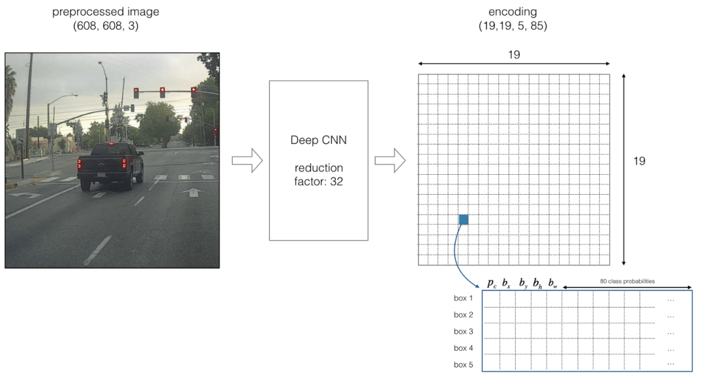
Let us examine below image to understand stride and structure of predictions better. Below stride is 32 and input image size is (608, 608, 3). Let us say we are dealing with Coco dataset that has 80 classes and are using a batch size of ‘m’. Then
(m, 608, 608, 3) -> CNN -> (m, 19, 19, 5, 85)
where 19, 19 is output feature map size (608/32 = 19), 5 is number of anchor boxes, and 85 = 80 classes + 5 bounding box coordinates

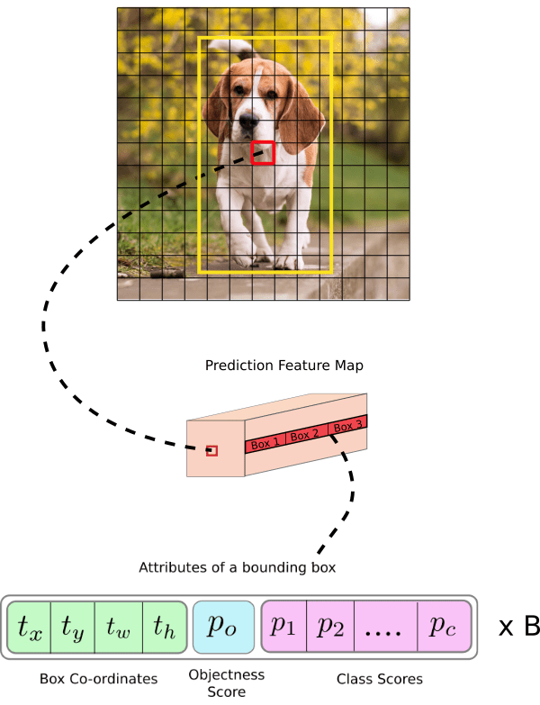
If center of an object falls on a particular cell (shown as blue in Fig-10), that cell is responsible for detecting that object. As we are using 5 anchor boxes, each of the 19×19 cells will carry information about 5 boxes. Structure of prediction vector for this will be as below.

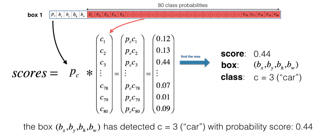
Now for each box (for each cell), predicted objectness score (Pc) is multiplied with class probabilities and max probability that comes out will be taken as the class of object detected. Refer below image.

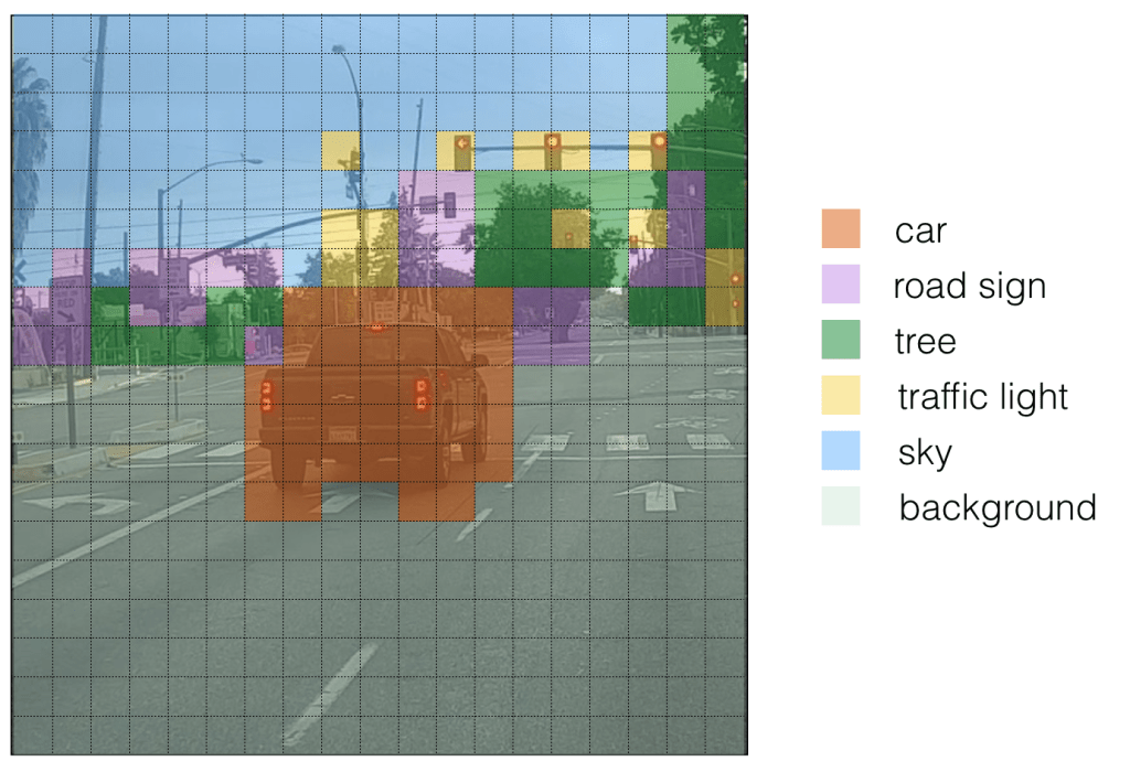
For ease of visualization let us assign different colours for each of the classes detected. Please note that this is not the output of Yolo but we can consider it as an intermediate state before non-maximum suppression (NMS).

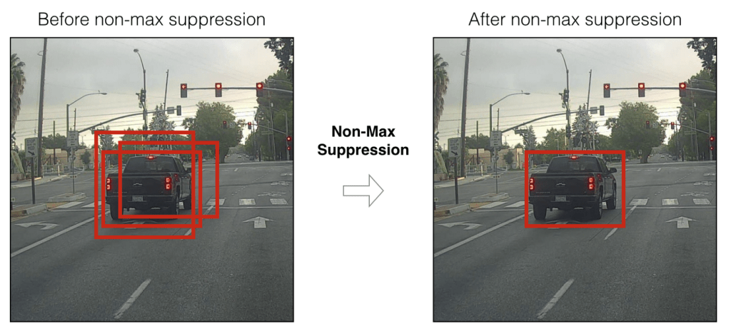
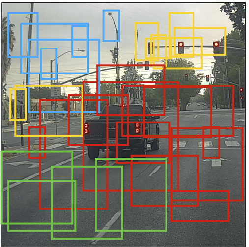
If we put bounding boxes around these objects, image will be as below. There are too many bounding boxes here but Yolo will bring down to 1 bounding box per object by using Non-Maximum Suppression (NMS).

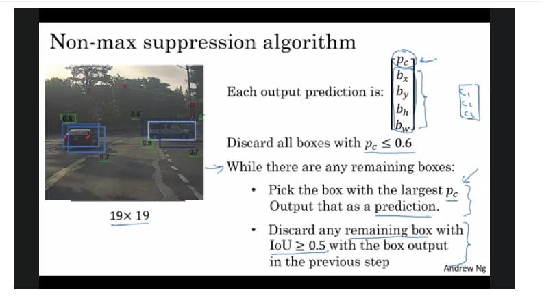
NMS : Below image shows how non-maximum suppression works & eliminates duplicate bounding boxes. Also refer the video link listed in source below to get a better intuition. Please note that Pc and IoU numbers given in below image are representative.

11. Center coordinates and Bounding Box coordinates

Why should Yolo predict scale by which anchor boxes need to be modified ? Why can’t it directly predict width and height of bounding boxes ? Answer – it is not pragmatic as it will cause unstable gradients while training. Instead, most modern object detectors including Yolo predicts log-space transforms or in other words – offsets and apply them to pre-defined anchor boxes. We already seen that Yolo predicts 4 coordinates around which bounding boxes are built. Following formula shows how bounding box dimensions are calculated from these predictions.

bx, by -> x, y center coordinates
bw,bh -> Width and height of bounding boxes
tx, ty, tw, th -> Yolo predictions (4 coordinates)
cx, cy -> Top-left coordinate of grid cell where object was located
Pw, Ph -> Anchor box width and heigth

Center Coordinates : Let us refer Fig-9. Dog is detected on (7,7) grid. When Yolo is predicting center coordinates (tx, ty), it is not predicting the absolute coordinates but offsets relative to the top-left coordinate of grid cell where object was located. Also these predictions will be normalized based on the cell dimensions from feature map. So for our dog image, if we get offset predictions as (0.6, 0.4) then in feature map it will be (6.6, 6.4). What if offsets predicted are 1.6 & 1.4 ? Coordinates will now be (7.6,7.4) taking object to grid location (8,8). But this breaks the Yolo rule which says cell that detected object (7,7) itself should be responsible for it. Hence we will pass the center coordinate predictions via sigmoid forcing the values to stay between 0 and 1 thereby keeping the grid location at (7,7) itself. As we covered equations 1 & 2 that gives bx, by let us move on to discuss bounding box coordinates.

Dimensions of bounding box (bw, bh) are obtained by applying log-space transformation to the predicted output (tw, th) and then mutiplying these with anchor box dimensions (Pw, Ph). This explains equations 3 & 4 above. These dimensions are normalized based on image height & width. This means if we get (0.3, 0.4) as output, in a 13×13 feature map, actual width and height of bounding box will be (13*0.3, 13*0.4). Below image visualizes the 4 equations given in Fig-15.

12. Yolo Loss Functions

Now let us take a look at loss function to understand how network trains and improves in object detection.

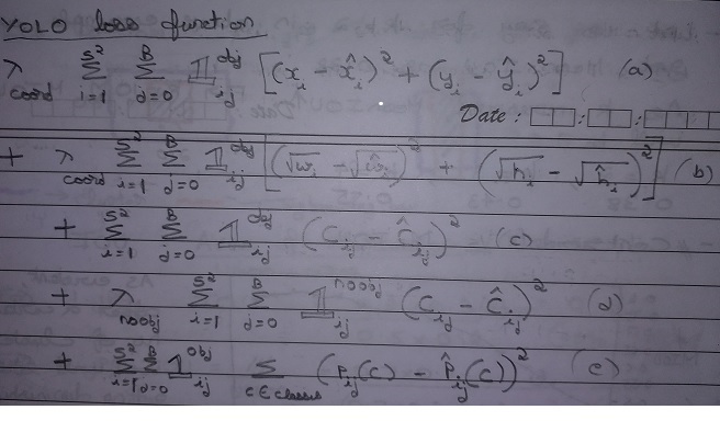
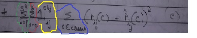
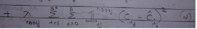
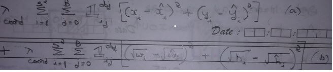
Yolo loss function is having 5 parts as shown in equation as a, b, c, d, e.

Let us start with (e) first. This part is dealing with classifying the object. This is same as the squared error loss functions used in image classification except the summations part and 1obj factor.

What we are doing via this equation is as follows. We are comparing the predicted class Pij(C)-Hat with ground truth Pij(C). We will do this for :

• Each cell in grid (green curve ) from 1 to 13^2, i.e for each of 169 cells. In our case S=13 hence 13^2.
• For each box inside each of the cells (red curve) i.e. 1 to B=5 as we are dealing with 5 anchor boxes
• For each class (Blue curve), if there are 80 classes then C = 80
• We will multiply each of the above occurrences with 1obj. This will help us to consider only those cells that is above a certain objectness threshold (section 5). More on this below.

Let us now examine (C). This part deals with cells that have object inside it.

• Summations and loop remains the same.
• Meaning of 1obj remains the same. Only those cells that are above the objectness threshold will get a value of 1obj as 1. Remaining all cells will have 1obj = 0 and will be ignored.
• For those cells with 1obj = 1, Cij (ground truth) will be assigned 1. This GT objectness score is compared with predicted objectness score Cij-hat
• Let us say in fig-9 only cell (7,7) met the threshold criteria and Yolo found that 3rd anchor has best IOU. Then only cell (7,7) i.e. i = 49 and anchor j=3 will have objectness score 1obj = 1.
• In other words i = 49, j= 3 instance of 1obj will be 1, all other occurrences 0.
• Let us say network predicted Cij-hat as 0.7 for this cell. Then loss value for this cell will be 1 * ( 1 – 0.7 )^2.

Next, let us see interpret (d). This part deals with cells having no-object inside it. It is equally important to assess & reduce false positives i.e. Yolo detecting an object when actually there is none. Part (d) serves this purpose.

• Summations and loop remains the same as in previous sections.
• Instead of 1obj we have 1noobj here. We will call 1noobj as No-objectness number. Here those cells that are above the threshold, will be assigned 1noobj = 0. This is because these cells have an object inside them. Remaining all cells will have 1noobj = 1.
• For earlier example, only for cell (7,7) i.e. i = 49 and anchor j=3 will have no-objectness score 1noobj = 0.
• In other words i = 49, j= 3 instance of 1noobj will be 0, all other occurrences 1.
• Yolo introduced one more factor Lamda-noobj in the equation. This is to mitigate the effect of (d) compared to (c).
• For (c) only 1 cell (or few cells) will be having value whereas for (d) most of the cells will have a loss-value. Loss-function value for (c) will be much lesser compared to (d). In our example while (c) has value only for 1 cell, (d) has value for all 844 cells.
• Hence network will ignore (c) and focus on reducing (d). But we want both objectness and no-objectness predictions to improve.
• Hence, we will reduce the effect of no-objectness (d) by introducing Lamda-noobj.
• We will give a lesser value of Lamda-noobj (0.0001) at beginning to make the value comparable with (c). As trainining proceeds, we will keep slightly increasing Lamba-noobj to ensure that it remains on par with (c).
• Let us say for cell, i = 56, j =2 network predicted Cij-hat = 0.3.
• We know that there is no object in this cell so Cij = 0
• Through (d), Yolo built a way to punish this and value of loss function will be 0.0001 * 1 * (0 – 0.3)^2
  where 1noobj = 1, Lamda-noobj = 0.0001, Cij = 0 (no-object in this cell)

Finally, let us see what (a) and (b) are meant for.

• This part deals with network learning about center location and bounding box dimensions.
• (a) deals with center location. xi and yi are ground truth coordinates supplied via training labels.
• xi-hat and yi-hat are network predictions that are compared with ground truth.
• (b) deals with bounding box width and height. wi and hi are ground truth dimensions supplied via training labels.
• wi-hat and hi-hat are network predictions that are compared with ground truth.
• We are using square root here to ensure that smaller bounding boxes are also optimized. Taking square root will magnify smaller errors & make them accountable.
  eg: Error = 0.0009 & Error ^ 0.5 = 0.03. If network encounters both these numbers, then it will prefer 0.03 over 0.0009 because 0.03 > 0.0009.
• There is a multiplication factor lamda-coord involved in both (a) and (b). In section 4, we mentioned “Initial epochs of Yolo network are trained only for classification.” lamda-coord is meant for this purpose.
• For initial epochs let us say 100 epochs, we will train only for classification and objectness. We achieve this by keeping lamda-coord = 0.
• In later epochs, we will train detection also by giving values to lamda-coord.

13. Network

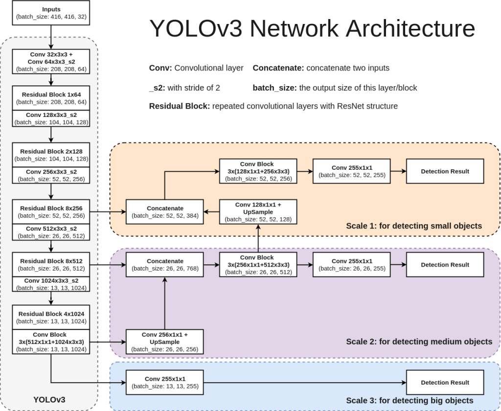
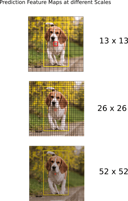
Each version of Yolo comes with its own modification in CNN network. For sake of understanding, we will refer Yolo V3 network here. Network used for Yolo V3 is Darknet-53. It uses only convolutional layers. Instead of max-pooling it uses 3×3 with a stride of 2. Also, network predicts at 3 feature map scales – 13×13, 26×26, 52×52. Lower feature map scales were introduced to detect lower resolution objects. Below architecture diagram is self-explanatory to understand the network. Also shown below is how feature map predictions at 3 scales will look like.
Standard metric used for evaluation of Yolo network is mAP – Mean Average Precision. You can refer below two articles to get a better understanding on mAP.
Medium_JonathanHui_map
tarangshah_map

14. Conclusion

That’s it for Yolo intuition. Yolo is rapidly evolving. At the time of writing this article Yolo V5 is already out and we can expect more versions to be released in future. I would recommend reading those papers and understand what is different from previous versions. Hope you were able to understand how Yolo works now and reading this article enable you understand future revisions.

In this article, we will discuss those components of Convolutional neural network (CNN) where prediction of images and feedback for those predictions happen. First, let us take a bird’s eye view on how CNNs work:
1) Input images in the form of tensors will be fed to CNN.
2) Convolution layers will extract features.
3) At the final layer, network will classify the object using the features extracted.
4) Back propagation will provide feedback to the network comparing predictions VS ground truth.
5) Network will update the weights of kernels based on the feedback.
6) Steps 1 to 5 will repeat till we train our network (epochs).

Activation Functions and why they are needed ?
Activation Functions are used in CNNs on step 2 mentioned above. Let us find out why they are needed and how it helps CNN ?
Convolutions are sum-products of tensors as shown below. This is essentially a linear operation that can be expressed in the form of w0*x0 + w1*x1 + ….

But real-life problems are non-linear. For example, if a car is about to hit us, we will instantaneously jump to safety. If we plot the speed of car VS response, the curve will be non-linear.
Hence for CNNs to deal with complex problems, sum-of-products(linear results) that convolutions provide are not enough. We apply activation functions on our convolution outputs to deal with this. Activation functions bring non-linearity to the convolution output. Below is a pictorial representation of the same. Output of activation function is fed to the next convolution layer.

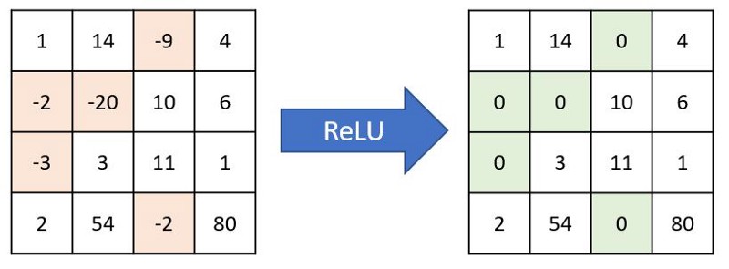
Most commonly used activation function is Relu (Rectified Linear Unit). Relu converts negative numbers to zeros and carry forward positive numbers. If a feature is not helping the network, then Relu won’t carry it forward (makes it zero), else carries it forward as such. Even though there are other activation functions like Sigmoid or tanh, Relu is preferred in most networks because of its simplicity and efficiency. Below is how Relu acts on a channel and gives back output.

Global Average Pooling (GAP)
To understand GAP concept, let us imagine a convolution layer trying to predict 10 different animals (10 classes). Below points should be kept in mind while we proceed.
a) For network to be effective, we should convolve till Receptive Field (RF) reaches >= image size.
b) Nodes in the final layer must be exactly same as number of classes we want to predict.
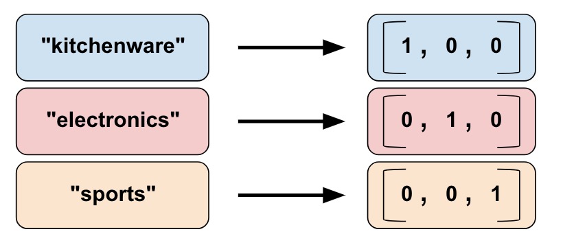
In this case, final layer passed to softmax for prediction needs to be 1x1x10. This 1x1x10 tensor is called one-hot vector because only one of the nodes (predicted class) will have value. An example for one-hot vector encoding is as below.

Lets us design convolution layers for our problem as below:
Layer 1 : 28 x 28 x 3 * 3 x 3 x 3 x 16, padding = True -> 28 x 28 x 16 (RF = 3)
Layer 2 : 28 x 28 x 16 * 3 x 3 x 16 x 32, padding = True -> 28 x 28 x 32 (RF = 5)
Layer 3 : 28 x 28 x 32 * Maxpooling -> 14 x 14 x 32 (RF =6)
Layer 4 : 14 x 14 x 32 * 3 x 3 x 32 x 32, padding = True -> 14 x 14 x 32 (RF=10)
Layer 5 : 14 x 14 x 32 * 3 x 3 x 32 x 32, padding = True -> 14 x 14 x32 (RF=14)
Layer 6 : 14 x 14 x 32 * Maxpooling -> 7x7x32 (RF = 16)
Layer 7 : 7 x 7 x 32 * 7 x 7 x 32 x 10 -> 1x1x10 (RF = 28)
Layer 8 : 1 x 1 x 10 * Softmax -> Predicted Output

Lets us focus on layer 7. This layer prepares data for final predictions. Here number of parameters involved will be 15,680 (7*7*32*10). This layer alone will make our model compute heavy.
In addition, by following this approach we have one more disadvantage. In layer 7, we are combining 32 channels to 10 channels. Ideally we can do this through 32*10 = 320 combinations. However by keeping prediction layer (layer 8) directly after layer 7, we are forcing 7x7x32 to act as a one-hot vector. This will cause 32 channels to be re-purposed solely for prediction purpose. Due to this, the combination is reduced from 32*10 to 32*1 limiting the ability to use features from 7x7x32 layer effectively. This scenario is shown in left part of below image.

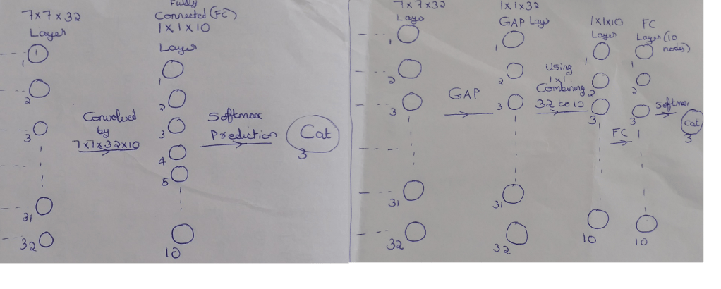
Now focus on the set-up shown in the right part of image.
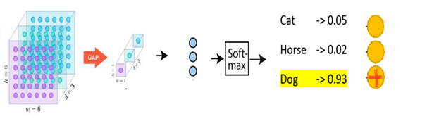
– We are doing Global Average Pooling (GAP) to convert 7x7x32 to 1x1x32. We are taking average of 49 values to reduce it to 1 value per channel. (Since parameters are not optimized, No: of model parameters = 0)
– Next we are combining the GAP output 1x1x32 using 1x1x32x10 to give 1x1x10. (No: of model parameters = 32*10 = 320)
– 1x1x10 is then connected to Fully Connected (FC) layer which is passed for Softmax prediction.
This approach takes out the pressure of one-hot encoding from 7 x 7 x 32 layer and enables the network to utilize layer 7 much better. Also, we have significantly reduced the model parameters with this approach. Below is an image showing GAP -> FC -> Softmax for prediction of 3 classes. Here GAP is converting 6x6x3 to 1x1x3.

Softmax
Softmax is a widely used activation function in CNN for image classification of single objects. Output of FC layer that we discussed above will be fed to Softmax. Below image shows where Softmax fits in a CNN architecture.

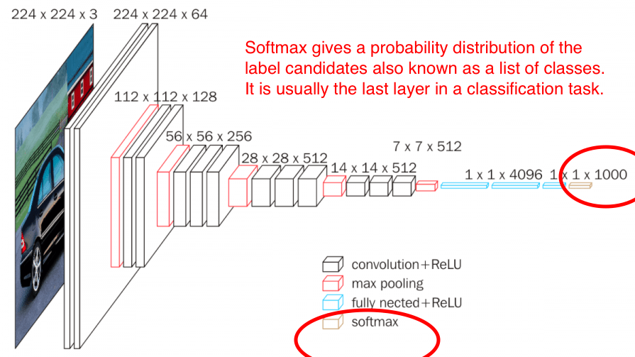
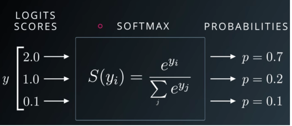
As seen above, Softmax is the final layer in CNN architecture and gives the probability distribution of list of classes. The class with the highest probability will be selected as the predicted class. The output of the softmax gives us the likelihood of a particular image belonging to a certain class. Formula for Softmax and how it helps predicting images is depicted in below snippets.

• In above image, each row shows probability of input image belonging to each of the 3 classes. Network predicts that it is a cat with 0.71 likelihood for first image.
• For second image, likelihood of the image being a horse is very high (0.98).

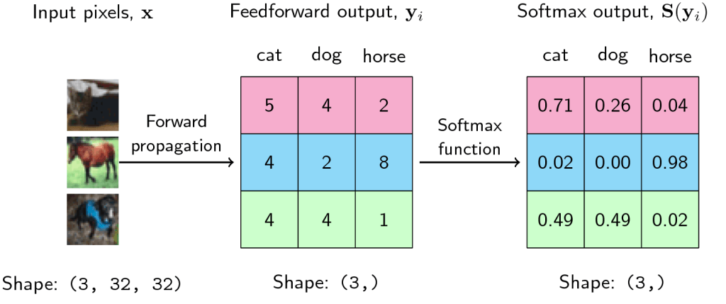
Let us inspect third scenario. Here likelihood of image being dog is same as that of cat (0.49). In reality these 2 numbers can never be same. Hence, it will be like probability of dog = 0.49001 and cat = 0.48999 or vice versa. Model will predict the class with higher probability. If model predicted that image is a dog, then prediction accuracy for this image is 100%. If it predicted cat, then accuracy drops to 0%. Margin between switching accuracy from 100% to 0% is very thin – 0.00002. Hence measuring accuracy alone can’t tell us how good our model is. We should be able to quantify how confident our model is about the class it predicted being true. This brings us to the concept of Negative Likelihood Loss.

What is Negative Likelihood Loss (NLL) and why is it required ?
We already seen that accuracy alone is insufficient to understand how good a model is. This becomes particularly important when predictions are made on the basis of a narrow margin. Let us take another example to further understand this concept.
Imagine there are 100 individuals in your village. An election is called upon to nominate the village head. Each of these 100 individuals stood as candidates for election. Incidentally 2 among them happens to be you and your spouse. Now all the remaining 98 individuals voted for themselves. You convinced your spouse to vote for you. When results are out, you won the elections. But the vote percentage you received is 2% compared to 1% for 98 others and 0% for your spouse. Here the result alone is not giving us accurate picture on how badly you won the elections.
This could happen in our CNN models also as seen in the dog vs cat example above. NLL gives us a measure on how confident a model is about predicting a class and hence throwing it out. It indicates the degree of confidence of model.

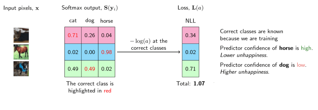
Formula for NLL is L(y) = -log(y) where y is prediction and L(y) is NLL.

Below is the softmax table modified after adding NLL values. As we can see, lower the NLL value, happier the model (degree of confidence : high).

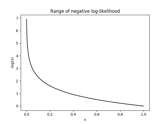
Graph for NLL is as follows. NLL becomes unhappy at smaller values, indicating that model is not predicting with enough confidence. It will become very sad (infinite unhappiness) when model confidence touches even smaller values. NLL becomes happy at larger x values indicating that model is predicting emphatically. What happens here is that in loss function, we will sum the losses of all the correct classes. So whenever the network assigns high confidence (x) for the correct class, the unhappiness (-log(x)) becomes low, and vice-versa.

Hope this article gave you an intuition on how final layers of a CNN operates and gives predictions.

In Deep Neural Networks, maintaining same image size throughout the network is not sustainable due to huge computing resource it commands. At the same time, we also need enough convolutions to extract meaningful features. We learnt in last article that we can strike a balance between these two by down-sizing at proper intervals. In this article, we will discuss on how down-sizing is done. We will also cover how to combine channels using 1×1 convolutions and discuss Receptive Field (RF) calculation.

Why we need Max-Pooling ?
3×3 convolutions with a stride of 1 increase RF by 2 (details on stride here). Also, for effective image classification, RF should be >= size of image. Let us take an image of size 399×399 and imagine we only have 3×3 convolutions at our disposal. How many convolution layers will it take to reach RF of 399 ? Approximately 200 layers as shown below. Such a network will require huge computing power for processing.
399 * 3×3 -> 397 ; RF = 3
397 * 3×3 -> 395 ; RF = 5
395 * 3×3 -> 393 ; RF = 7
393 * 3×3 -> 391 ; RF = 9
391 * 3×3 -> 389 ; RF = 11
.
.
5 * 3X3 -> 3 ; RF = 397
3 * 3X3 -> 1 ; RF = 399
Hence, we need max-pooling to down-size the channel size at proper intervals so that we can get the job done within manageable number of convolutional layers. Below is how it looks like with max-pooling. We are reaching RF >= 399 in 30 layers (we will cover RF formula later).
399 | 397 | 395 | 393 | 391 | 389 | MP (2×2)
194 | 192 | 190 | 188 | 186 | 184 | MP (2×2)
92 | 90 | 88 | 86 | 84 | 82 | MP (2×2)
41 | 39 | 37 | 35 | 33 | 31 | MP (2×2)
15 | 13 | 11| 9 | 7 | 5 | 3 | 1

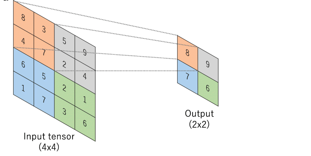
What is Max-Pooling ?
Max-Pooling is a convolution operation where kernel extracts the maximum value out of area that it convolves. Below image shows Max-pooling on a 4×4 channel using 2×2 kernel and stride of 2.

How to do Max-Pooling ?
Common practice is to use 2×2 kernel with a stride of 2. However kernels of any size can be used. We will get a single value out of the area covered. Hence bigger the size of kernel, higher the number of pixels getting omitted. Let us look at below scenario:
2×2 -> 1 out of 4 values selected
3×3 -> 1 out of 9 values selected
5×5 -> 1 out of 25 values selected
Bigger the kernel size, faster the compression. This may not be prudent. Hence most of the networks prefer 2×2 Max-Pooling with a stride of 2. Just to give you an intuition of how extraction happens, below is the image of 3×3 Max-Pooling with a stride of 3 .

When to use Max-Pooling ?
Rapid down-sizing is not sensible. It will lead to downsizing without extracting anything meaningful. Hence we should Max-Pool only at proper intervals. These intervals will vary based on the complexity of input images.
For example, in case of simple images like hand-written digits, we can Max-Pool at an interval of 5 RF i.e. 3×3 -> 3×3 -> Max-Pool. Whereas for complex problems like emotion detection we have to Max-Pool at higher RF intervals like 11 or more.
3×3 -> 3×3 -> 3×3 -> 3×3 -> 3×3 -> MP
This is because for hand-written digits even at an RF of 5, network should be able to extract meaningful features. But in problems like human emotion detection, input image is more complex and hence network has to convolve more to extract meaningful features. In this case, if we apply Max-Pool at RF =5, we will start down-size even before any meaningful extraction. It will be akin to downsizing a product team before development completion.

By omitting pixel values are we reducing our opportunity to learn more ? As discussed in earlier point, we start Max-Pooling only once we get a confidence that meaningful features are already extracted. By following this approach, we will be able to retain the relevant features and make them available for future layers to learn.
Retaining all the pixel values may help network to learn more but is it really required ? In most cases, no. If we can accurately detect an object with lesser parameters, we should go for it rather than over-learning and waste resources.
In addition to the above point, removing irrelevant features are equally important. eg: background in a dog image need not be carried forward. Through Max-Pooling we are accomplishing this objective too.
Why we take maximum value ? This is to ensure that most prominent feature is carried forward for future layers of network to learn. In CNN convention, bigger the channel value more important the feature. Through back-propagation, network will ensure that prominent features are getting higher values.
Eg: If the door knob of a house is important in an image classification problem, then irrespective of size of door knob compared to overall image, network will ensure that it gets carried forward till final layer. Network does this by assigning higher values to associated features.
What if all the values are similar ? Makes our life easier. This means, all the features in those channels are similar and we are just picking most relevant out of these similar features.

Below image shows how Max-pooling works in digit recognition problem. We can see that bigger pixel values are carried forward without losing any spatial information (8 still looks 8).

1 x 1 convolutions

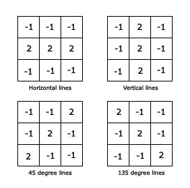
In CNNs, we generally extract features using 3×3 convolutions. We store these features in separate channels like vertical edge in one channel, 135 degree edge in another etc.

While convolving, the approach we use is as follows – start with smaller number of channels and then increase number of channels. Rational is to start with simple features like edges and gradients which will be stored in lesser number of channels. Then we will build complex things like patterns, textures, part of objects etc. out of these simple features. We will store these complex features in variety of ways using higher number of channels.

Let us try to understand how 1×1 convolutions helps our above approach, by examining Squeeze-expand (SE) architecture. Please note that use of 1×1 convolutions is not limited to SE. We are just using SE here to understand the concept. Squeeze expand architecture increases number of channels step-by-step each block. When next block starts, we again start with smaller number of channels and keep increasing channels step-by-step.
Below is an example of squeeze expand network:

We will be focusing our discussion on the highlighted operation. Before we start, please keep below two points in mind. For more details on these, refer here.
a) No: of channels in kernels need to be same as number of channels in input
b) No: of kernels we want to convolve depends on number of channels we want in output.

Let us understand what is happening above:
392x392x256 | (3x3x256)x512 | 390x390x512 RF of 11X11
CONVOLUTION BLOCK 1 ENDS
TRANSITION BLOCK 1 BEGINS
MAXPOOLING(2×2)
195x195x512 | (1x1x512)x32 | 195x195x32 RF of 22×22
TRANSITION BLOCK 1 ENDS

First convolution
392x392x256 | (3x3x256)x512 | 390x390x512 RF of 11X11
Here 256 channels of 392×392 size are convolved by 512 kernels of size 3x3x256 to get 512 channels of 390×390 (No padding).
Second convolution
MAXPOOLING(2×2)
Max-Pooling using 2×2 kernel with stride 2 to get back 512 half-sized channels i.e. 512 channels of 195×195 size (half of 390×390).
Third convolution
195x195x512 | (1x1x512)x32 | 195x195x32 RF of 22×22
Here we are combining 512 channels of 195×195 size using 32 channels of size 1x1x512 to get back 32 channels of size 195×195.

Essentially the purpose of 1×1 convolution is to combine channels to give richer channels. What do richer channels mean ? Let us say we have 3 channels – one stores left eye, second stores right eye and third stores forehead. What 1×1 can do is combine all these 3 channels to give back a single channel that stores upper portion of human face.

1×1 retains height (H), width of channel while combining depth (D) to single pixel. Below is an example of single 1x1xD kernel convolving on D channels of size HxW to give back a single HxW channel. Here 1×1 is combining D channels to a single channel.
HxWxD | 1x1xDx1 | HxWx1
Why 1×1 has D channels (1x1xD) ?
Because input channel has D channels (HxWxD). No: of channels in kernels need to be same as number of channels in input.
Why we are using only 1 kernel (1x1x10x1) ?
Because we need only 1 channel in output for this particular case. No: of kernels we want to convolve depends on number of channels we want in output.

Let us look at one more example. Image below shows four 1x1x10 kernels convolving over 10 channels of 32×32 size to give back four channels of 32×32 size.
32x32x10 | 1x1x10x4 | 32x32x4
Here 1×1 is combining 10 channels to 4 channels.
Why 1×1 has 10 channels (1x1x10) ?
Because input channel has 10 channels (32x32x10). No: of channels in kernels need to be same as number of channels in input.
Why we are using 4 kernels (1x1x10x4) ?
Because we need 4 channels in output for this particular case. No: of kernels we want to convolve depends on number of channels we want in output.

1×1 calculations : Below image will give an idea on calculations that happen while using 1×1 convolutions.

– In first set, 6x6x1 is convolved by a single 1x1x1 kernel to give back 6x6x1. Please note that 1x1x1 kernel is a single value & in this example its value is 2.

– In second set, 6x6x32 is convolved by 1x1x32 kernel. Here # of kernels is kept open. 1x1x32 will be having 32 values across the depth. Each value in the 6×6 channel across the depth will be multiplied by its corresponding 1×1 kernel value and all these will be combined to give a single cell. This way we will get 6x6x(# kernels) in return. Please refer the image “1×1 convolution HxWxD | 1x1xD | HxWx1” if you want help visualizing this.

Another important advantage of 1×1 convolution is that it reduces burden of channel selection from 3×3.
Example : We want to predict dog, cat and tiger from a set of images. We gave image of tiger as input. In a particular layer we are at 28x28x256 channel size and want to get 16 channels out of this convolution. We only have 3×3 at our disposal. In this case, 16 different 3x3x256 kernels has to convolve to give 16 channels. Not all these 256 channels from input will be relevant for tiger. But 3×3 can figure this out only based on feedback it receives from back-propagation.
Suppose in this case, we are allowed to use 1×1. Then, we can combine our 256 channels to 16 channels using 1×1 convolution and pass only 16 channels for 3×3. In this case, only 16 different 3x3x16 has to convolve on 28x28x16 channel. We are significantly reducing number of parameters in the latter case.
This makes network faster as 3×3 can now decide relevant tiger channels from 16 instead of 256.

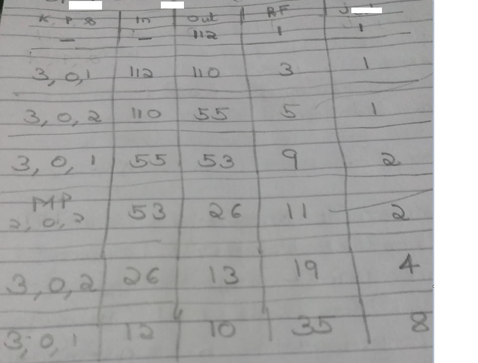
Receptive Field Calculation
Before we wrap-up this article, let us check the way in which we calculate the RF.
Below is the formula for the RF. Note that r -> RF , j -> jump

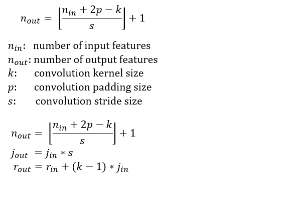
Attached below is a sample calculation so that we can understand how the formula works. Few points to note while going through below table. Write down Jump-out of layer 3, while doing calculations of layer 2 and so on.
For Layer 1 : Jump-In = Jump-out = 1, Out = Input Size
For Layer 2 : Jump-In = Jump-out of layer 1
Jump-Out = Jump-In * stride
For Layer 3 : Jump-In = Jump-out of layer 2
Jump-Out = Jump-In * stride
………….
………….
For Layer 1 : RF-In = RF-out = 1
For Layer 2 : RF-In = RF-out of layer 1
RF-Out = RF-In * stride
For Layer 3 : RF-In = RF-out of layer 2
RF-Out = RF-In * stride
………….
………….

---

---

---

---

---

This article is continuation of my article that you can find in below link.
Deep Learning- Understanding Receptive field in Computer Vision

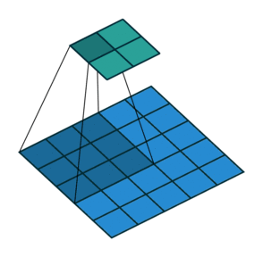
In last article, we mentioned that convolutions are the key operations that enable Convolutional Neural Network (CNN) to extract features, create various channels and thereby increase receptive field (RF). In this article, we will check how convolutions performs these. Below is an animated image of 4×4 convolved by a 3×3 kernel to give 2×2 channel. Channels are the output of convolutions. Convolutions extract features and save it in channels. Channels are also called feature maps.

Let us look at an analogy to understand channels better. Imagine a musical band playing. We can hear song along with sound of musical instruments. All these in harmony only will make the performance worth listening. Now imagine the components of this musical play like human voice, guitar, drums etc. Each of these components when extracted and stored can be called as channels/feature maps.

How values are populated in channel cells via convolutions is as shown below. Below example is without padding.

Padding
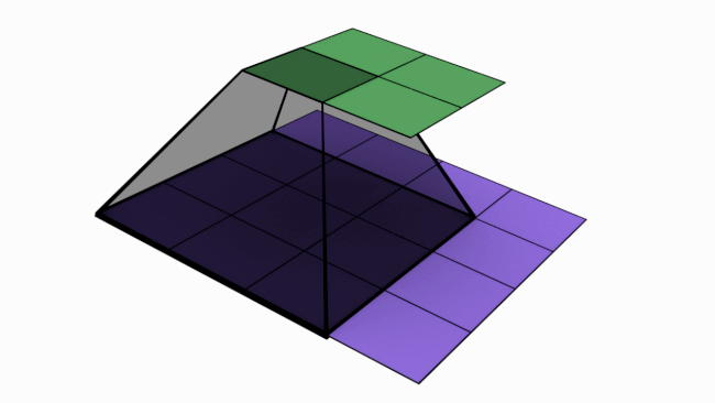
In the first animation, if you noticed, all the pixels are not convolved same number of times. Only the central pixel is covered 9 times. Rest of the pixels are convolved lesser times. If we are not retaining the size, box will keep shrinking and central portion getting covered 9 times (when we use 3×3 kernel) also will shrink accordingly. If we are not convolving enough times CNN may not be able to extract all required features. Below is an image of padding = 1 applied on 6×6 image.

One of the advantages of using padding is that we can retain the central portion available for convolutions. Padding means adding additional columns and rows on borders. Though in above image we filled padded rows and columns with zeros, in general we fill them with border values. Please check the below image to understand how central portion increases as size increases.

However in previous article, we seen that retaining same size throughout is not viable. So how will we solve this problem – i.e. retaining the size vs reducing the size progressively ? We can achieve this by using blocks and layers as explained below.

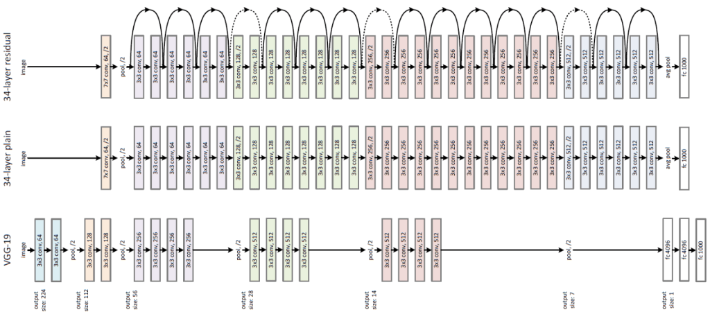
Please check the middle one in above diagram (34-layer plain). What you are seeing is a model architecture that has 4 blocks with 6 layers, 8 layers, 12 layers and 6 layers respectively. You can identify these blocks based on color change. Here, we are retaining same channel size per block using padding. At the end of each block we will down-size the channels using an operation called Maxpooling. Channel size reduction per block will happen something similar as below:
Block 1 -> 56×56
Block 2 -> 28×28
Block 3 -> 14×14
Block 4 -> 7×7
Disclaimer : There are other purposes also behind keeping block-layer architecture and using padding. But more on it later.

But how convolutions are extracting features ?
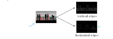
Let us understand this with a simple example. Feature extraction starts with basic edges/gradients and then these features are convolved to create more complex features like patterns, parts of objects and objects. Let us see how convolutions extract a vertical edge. Please note that higher numbers in below example represent brighter pixels i.e. 10 will be brighter than zero. An edge is detected when there is a sharp change in pixel values.

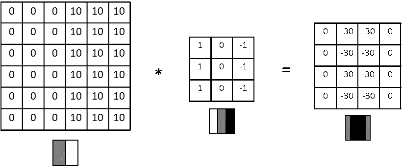
Here a 6×6 input is convolved with 3×3 kernel to give a 4×4 channel output. The values that you are seeing inside kernel are called weights. Now let us inspect what is happening from a physical sense.
6×6 input -> Imagine this as a portion of image where a vertical edge is there. Like the wall of a building where there is sudden transition from wall (dark pixels) to outside sunny world (bright pixels). You can see the values stacked up as 0s on left and 10s on right.
3×3 kernel -> Rather than seeing this as a kernel, imagine this as a feature extractor. In this case, our feature extractor is specialized in vertical edge extraction. How ? Please notice the weights inside this kernel. We have a bright left column (pixel values 1), then a dark middle column (pixel values 0) and finally a darker right column (pixel values -1). Basically kernel weights are build in such a way that it is transitioning from bright to dark to darker.
Output -> We have already seen how sum of products happen during convolution and how we arrive at output channel values. Interesting thing here is we extracted a vertical dark edge using above convolution. Check the image above. We got a 2 column width dark edge extracted and stored in a 4×4 channel (feature map). Follow-up question : How we got a much darker edge in output, when input edge was not this dark ? Answer : We increased the amplitude of dark edge we seen in input so that it won’t get diluted in future convolutions.
View more examples of edge extractors as below.

Below image will help you to visualize how edges play a role in an image.

What are strides ?
Stride is the number of pixels that shift over when kernel convolves over input. Strides plays a role in determining output channel size as well as receptive field. In first image we seen stride of 1. Below is a convolution with a stride of 2.

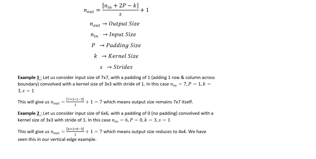
Since we now understand what is stride and padding, let us generalize the output size as below.

Convolution with multiple kernels to give multiple Channels
So far we have seen convolutions with one kernel to give one channel i.e. we were discussing in 2D like 7×7 * 3×3 -> 5×5. But in real networks, we create multiple channels layer-by layer or block-by-block. In below image you can see channels increasing in the order 1 – 25 -25 -32 -32 – 64.

Let us inspect this in detail. We need to note below points while convolving with multiple kernels to get multiple channels.
– No: of channels in kernels need to be same as number of channels in input
– No: of kernels you want to convolve depends on number of channels you want in output.
For example:
28x28x3 * 3x3x3x32 -> 26x26x32
28x28x3 -> Imagine this as 28×28 dimensional matrices stacked one on top another 3 times. Rectangular prism with l, w =28 & depth = 3
Kernel size -> 3x3x3 Imagine this as 3×3 dimensional matrices one on top of another 3 times. Like a cube with all sides as 3.
Here no: of channels input (3) = no: of channels in kernel(3)
3x3x3x32 -> We are using 32 such types of 3x3x3 kernels
28x28x3 * 3x3x3x32 -> This means we are convolving 28x28x3 with 32 different types of 3x3x3
Result is 26x26x32 -> We will get 32 channels of 26×26 size
Here no: of kernels we used in convolution (32) = No: of channels in output (32)

Below is an animated representation multiple kernels convolving to give multiple channel outputs. Here input is 5x5x3. As input channel size is 3, we need to have 3 channels in kernel as well. We are using a 3×3 kernel here. So after considering the number of channels also, we can call it a 3x3x3 kernel. We are using 4 such kernels which makes it 3x3x3x4. We are convolving 5x5x3 with 3x3x3x4 to give us 3x3x4 outputs i.e. 4 channels of 3×3 size. (No padding used)

You can understand the calculations behind this by going through the image below. Here a 7x7x3 is convolved by 3x3x3x1 to give a 5x5x1 output.

In next article, we will discuss about down sizing the channel size through maxpooling which is another type of convolution.

In last week article, we got a high level view on how neural networks identify objects. This week, we will cover items that will help us understand the concept of receptive field and why it is important in neural networks. You can find my last week article here.

What is receptive field (RF) ? Let us look into the below image.

For sake of understanding, imagine the animation above as a simple neural network. There are 3 layers in this network 5×5 -> 3×3 -> 1×1. Notice the dark shadowed box moving over the pixels. This operation is called convolution. The blue square grid is input image with size 5×5. Box with shadow that is moving over image is called kernel (in this case size 3×3). We can see that 5×5 convolved with 3×3 kernel gives us 3×3 output (yellow). Yellow 3×3 when convolved again with 3×3 kernel results in 1×1.

Receptive Field is a term used to indicate how many pixels, a particular pixel in a layer has seen in total – both directly and indirectly. There are two kinds of RF – local and global. Local RF refers to the size of kernel. Global RF is what we commonly refer to as RF.

Let us take a closer look to understand what this means.

Layer 1 (Blue) : Each of the 25 pixels know only about itself. GRF = 1

Layer 2 (Yellow) : Each of the pixel have seen 3×3 pixels from layer 1 and hence knows them. Notice how the darker shades over blue panel translates to a single cell in yellow panel. Here GRF = 3

Layer 3 (Green) : There is only 1 pixel. This pixel has directly seen 3×3 pixels from layer 2 and knows them. But each of these layer 2 pixels already have info about 3×3 pixels from layer 1. Hence layer 3 pixel has indirectly seen all the 5×5 pixels. Hence GRF = 5. Keep in mind that our original image size is 5×5.

Relevance of receptive field

Computer vision networks that we are discussing belong to supervised learning models. We will feed labelled images (training set) to the model and make the model learn. Then we will feed the model with test images. We know the labels for these test set but we won’t tell that to model. Instead, we will ask model to predict based on what it learnt. Based on prediction vs ground-truth, we determine the accuracy of model. In the training process, neural networks will check the label (dog, cat etc.) and learn the characteristics for a particular object. After training on enough variety images, model will acquire enough knowledge to classify a dog as dog. This model once it identifies the characteristics of dog in a given image will be able to classify image as dog correctly.

We help the network learn by breaking down images to tensors and then reconstructing again step by step as shown below. Detailed explanation is in my article.

• We will break down image into basic channels.(We will cover channels later)
• The features inside these channels are then used to construct edges and gradients.
• Using these edges and gradients, we construct textures and patterns.
• From these textures and patterns, we build parts of objects.
• These parts of objects will be used to build objects.

In the above process of reconstruction, we are gradually increasing the RF of our network layer-by-layer. One point to note is that final layer RF must be = or > than size of original image. Let us understand this concept by answering few questions as below.

Why we need RF in final layer > or = to size of image ?
As we have seen, each pixel in a particular layer sees the world via pixels of its preceding layer. If you remember, final layer feeds the data to Softmax layer for classifying the object. Hence in order to share relevant data for classification, pixels in final layer must have seen the whole image. Imagine being tied to your seat in a theater and neck locked with blinders in such a way that you can see only in a straight line. Then you are asked to explain what is happening in movie. Obviously you wont be able to comprehend much visually. Same case applies to our final layer as well. We shouldn’t expect our network to predict a cat by only seeing let us say its tail or legs. This is the reason why we keep RF of final layer > or = to size of image. This way whole image gets captured in terms of RF in final layer.

Won’t reduction of size i.e. 5×5 -> 3×3 -> 1×1 be a problem ?
While increasing the RF, we reduce the size but still retains vital information. We are filtering useful information and keeping them in different channels. Imagine a box with 10 different masalas. We can combine them to make let us say 1000 different dishes. Here we started with 10 channels and went on to create 1000 unique channels. Similarly we are breaking down original image to edges & gradients (masalas) and then combine them to create more complex channels (dishes) at later layers. These complex channels eventually help us in classifying the objects via softmax.
Disclaimer : We will maintain the size same in each block via padding. But we will cover blocks and padding as we advance in future.

What is preventing us from maintaining original size throughout ?
Snippet below shows 3 channels (RGB) each of size 4×4. Number of parameters involved = 4x4x3 = 48

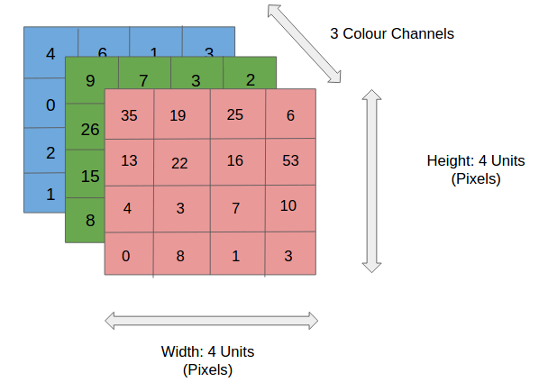
At each layer, we can define as many channels as needed for network to gain better accuracy (32, 64, 128, 256 etc). Imagine 400×400 matrix maintained for 1024 channels in a single layer. This single layer alone will need 163 million parameters. DNNs can have more than 100 layers in certain networks. Hence maintaining same image size throughout the network won’t be sustainable because of huge computing power it demands. Also as discussed above, it is not required to get our job done.

Before we wrap-up this article, let us answer one more question . What is the role of convolutions here ? Convolutions help us perform the operations we mentioned above – increasing the RF as well as creating various channels. I will be covering convolutions in upcoming articles.

Below is a neural network where you can see number of channels increasing layer-by-layer and you can see why maintaining high channel size is not a good idea.

In this article, I will share my understanding on how computers identify objects (Object classification) from images using deep learning. This article is from a birds eye view. I will continue to share more detailed views on various components involved in upcoming articles.

Let us start with difference between image and object from a computer-vision context.

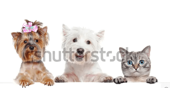
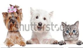
What we see above is an image. We can see 3 objects inside – 1 cat and 2 dogs. If we wish, we can count the ribbon on head of left one as 4^th object.

There are mainly 2 types of images – Red Green Blue (RGB) scale and gray scale (black & white) as illustrated below.

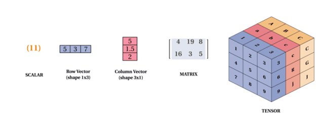
Unlike us, computers understand only language of mathematics. Hence we convert images to tensors using libraries like Python Imaging Libraries (PIL). You can imagine tensors as n-dimensional matrices as illustrated below.

So, how computers detect and classify objects ? One way in which computers achieve this is via neural networks. Below is a high-level representation of how neural networks work.

Lets us go step-by-step to understand the above flow. Please notice that lightning effect is going back and forth.

First let us understand the forward flow.

• Input images are converted to tensors and fed to neural network.
• These are then broken down to basic channels with a mathematical operation called convolution. You can imagine this like dismantling an assembled lego board to smaller pieces.
• We will then continue apply convolutions to our basic channels. This way we will reconstruct edges & gradients, textures & patterns, parts of objects and objects. These will happen inside hidden layers.
• In above diagram, we have shown only 1 hidden layer, but that won’t be the case in real models. We will have multiple hidden layers before final output layer. Towards the final hidden layers we can expect channels resembling original object that we are attempting to classify. (As shown below).
• Next we will flatten the output of final convolution layers and feed it to Softmax activation function. Dimension of flattened array will be same as number of classes. For example, if we want to predict digits (0-9), then softmax input will a 10 member array.
• Softmax will give us the probability of input image belonging to each class. Eg: cat : 0.05, dog : 0.92, horse : 0.03. Here predicted class is dog.

The steps I mentioned above comprise a forward pass. Next let us inspect what happens backward. We call this backward propagation. This is how model learns and improves.

• After prediction, each layer will receive feedback from its preceding layer. Feedback will be in the form of losses incurred at each layer during prediction.
• Aim of algorithm is to arrive at optimal loss. We call this as local minima.
• Based on the feedback, network will adjust itself so that convolutions will give better results when next forward pass happens.
• When next forward pass happens, loss will come down. Again, we will do backprop, network will continue to adjust and process repeats.
• This forward pass followed by back prop will keep happening the number of times we choose to train our model. We call it epochs.

Hope this gave you a high-level understanding on how a deep learning neural network detects objects. In future weeks, I will delve deep into the points mentioned above.

This is an example post, originally published as part of Blogging University. Enroll in one of our ten programs, and start your blog right.

You’re going to publish a post today. Don’t worry about how your blog looks. Don’t worry if you haven’t given it a name yet, or you’re feeling overwhelmed. Just click the “New Post” button, and tell us why you’re here.

Why do this?

• Because it gives new readers context. What are you about? Why should they read your blog?
• Because it will help you focus you own ideas about your blog and what you’d like to do with it.

The post can be short or long, a personal intro to your life or a bloggy mission statement, a manifesto for the future or a simple outline of your the types of things you hope to publish.

To help you get started, here are a few questions:

• Why are you blogging publicly, rather than keeping a personal journal?
• What topics do you think you’ll write about?
• Who would you love to connect with via your blog?
• If you blog successfully throughout the next year, what would you hope to have accomplished?

You’re not locked into any of this; one of the wonderful things about blogs is how they constantly evolve as we learn, grow, and interact with one another — but it’s good to know where and why you started, and articulating your goals may just give you a few other post ideas.

Can’t think how to get started? Just write the first thing that pops into your head. Anne Lamott, author of a book on writing we love, says that you need to give yourself permission to write a “crappy first draft”. Anne makes a great point — just start writing, and worry about editing it later.

When you’re ready to publish, give your post three to five tags that describe your blog’s focus — writing, photography, fiction, parenting, food, cars, movies, sports, whatever. These tags will help others who care about your topics find you in the Reader. Make sure one of the tags is “zerotohero,” so other new bloggers can find you, too.