Understanding Object detection with YOLO

YOLO – ‘You Only Look Once’ is state of art algorithm used for real-time object detection. Since its inception Yolo went through several revisions and latest version Yolo V5 was launched few weeks back. This article is not specific to any version but will give an overall idea how Yolo works. Aim of this article is to develop an intuition how Yolo detects an object which in turn will help understand the official Yolo papers and future revisions.

1. Let us start with Classification vs detection

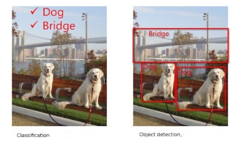
Classification tells us the object classes present in image whereas detection gives us the location + class names. We call those rectangles that show the location of the object – Bounding Boxes (BB).

2. Predictions in object detection

Object classification only has to tell us which object a particular image contains – dog, bridge etc. However, job of object detection is more tough. It has to predict the class as well as show the location. As shown below, algorithm should detect object/s and bound each of them – in this case person, bottle, laptop and chair.

For object classification, one hot vector prediction will be as follows for the above image:
Person – 0, One hot vector : [1,0,0,0]
Bottle – 1, One hot vector : [0,1,0,0]
Laptop – 2, One hot vector : [0,0,1,0]
Chair – 3, One hot vector : [0,0,0,1]

For object detection, prediction should include BB coordinates as well. Network needs to predict a minimum of 5 parameters – x, y (centroid coordinates of object), w, h (width & height of BB) and class. A network will predict accurately only if we train it properly. Hence for object detection network, training labels need to have following parameters – x, y (centroid coordinates of GT), w, h (width & height of GT BB) and class. We will see how Yolo predicts later in this article. * GT – Ground Truth

3. Quick recap – Object classification

Let us take a look at how object classification works via CNN.
– Convolutions are performed on original image.
– Image is broken into edges & gradients.
– Patterns are reconstructed from these edges & gradients.
– Then part of objects and eventually objects are reconstructed.
– If we convolve further, scenes are reconstructed.
Just before GAP layer, neurons will light up as below. ( Unlike below, size of final feature map may be smaller than the original image size depending on the network stride. eg: Image Size: 416, stride : 32, then final feature map size = 416/32 = 13)

Few pixels will be brighter than remaining pixels like the one that is bounded in above image. What this means is network found this particular feature strongly correlated with the class it is going to predict. For example, nose of dog could be the feature that network found unique for the dog class. These pixel/s are of great importance for Yolo.

4. Basic Idea – How Yolo Predicts ?

Initial epochs of Yolo network are trained only for classification. For subsequent epochs, both detection and classification are trained. During initial epochs network is just learning about the object it has to classify. Hence, it doesn’t make sense to ask the network to predict the BB at this point when it is not even certain about the object. As we have seen above, once network becomes adept at classification, some pixels will light-up more than others as we have seen above. Yolo will take the brightest pixel among these, find its centroid and put a bounding box around it. This is the basic idea how Yolo detects objects. Let us dive deeper to understand how this is done.

5. Objectness – How Yolo determines brightest pixel/s ?

Let us understand how Yolo identifies the brightest pixel/s so that network can focus only on those and ignore the rest. Yolo will break the image of size let us say 416×416 to a grid of fixed size say 13×13 (Why 13 x 13, we will see in section 10). As network trains in classification, it starts assigning a parameter called objectness score (OS) to all the cells.

Objectness means how much probability does a cell thinks it has an object inside it. Once OS is assigned, Yolo will filter the cells based on an objectness threshold. Let us say threshold is set at 0.8. Only those cells that have OS > threshold will be considered for further analysis. Yolo achieves this by assigning a parameter called Objectness number (1obj) to each cell. Those cells having OS above threshold will be assigned a value of 1 for 1obj. For all other cells Objectness number will be set to 0. Let us say in our 13×13 grid, only 2 cells qualified the OS threshold. Then only these 2 cells will be assigned 1obj value of 1 , remaining 167 cells will be assigned 1obj = 0. We will understand how 1obj helps to ignore below threshold cells once we examine the Yolo loss function.

Let us say 3 cells qualified. This could mean two things:
1) There were three objects as in fig-1 i.e. 2 dogs and a bridge. If so, we are good.
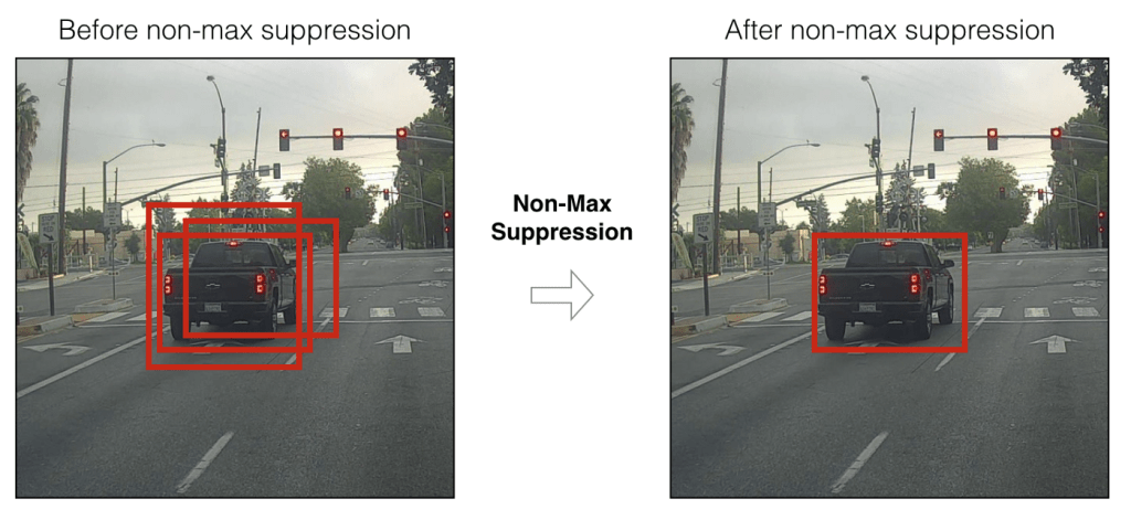
2) But what if image has only object. This means adjacent cells belonging to the same object passed the objectness threshold. In such a case, Yolo will choose the best cell out of these 3 based on a method called Non-Maximum Suppression(NMS) with the help of objectness score and IOU. More on these later.

6. Anchor Boxes in Yolo

Yolo network mainly has 2 tasks – classification and detection. As mentioned earlier, detection means detecting the location of centroid and BB width and height. Yolo uses concept of anchor boxes to bound the object. So, what are anchor boxes and why are they needed ? Each object is unique and will have its own size and shape. Box that can bound a bird may not be able to bound a car. So, bounding boxes will differ based on the object class as well as pose. Instead of creating a bounding box on the fly during training, Yolo uses fixed number of template boxes (3 or 5) that we call anchor boxes (priors – in official paper). How this fixed number is arrived ? We will see in Section 7.

Imagine packing your household items as part of shifting home. Creating a customized box for each item will end-up creating 100s of boxes. So pragmatically, we select few template boxes in which we will pack the things. Let us say your television set doesn’t fit to any of the templates. You found one of the templates slightly big but closely matching. You will use this template but fill the extra spaces with thermocol or clothes so that TV will stay tight. Similar concept is used in Yolo. In Yolo, we will use anchor boxes to bound the objects. These anchor boxes wont be perfect fit for the objects that Yolo detects. Hence as seen with TV set, Yolo will choose the best matching anchor box and scale it appropriately to bound the object. Yolo V2 uses 5 anchor boxes while Yolo V3 used 3 anchor boxes. In this article, we will stick on with 5 anchor boxes.

In order to scale the anchor boxes, we need some factor by which dimensions should be scaled. From where we get these scaling factors ? Answer – network will predict the factor by which anchor box height and width need to be scaled up/down. Based on these predicted factors, Yolo will scale the anchor boxes thus giving us bounding boxes.

7. How to select the best bounding box ?

As decided in prior section, we will use 5 anchor boxes in this article. What this means is that for each cell, network will predict 5 boxes. Based on objectness number, objectness score and using NMS, network will filter down the number of cells to one cell per object. This cell will have 5 bounding boxes corresponding to the 5 anchor boxes we are using. But we need only 1 box to bound an object. How Yolo chooses 1 out of these 5 boxes ? This is where IOU comes into picture. As we have seen in section 2, training labels that we supply for Yolo will have ground truth for class, object centroid location & bounding box width and height. Based on these ground truth coordinates, we will get ground truth bounding box area. Yolo will predict centroid locations and scaling factors for each of 5 anchor boxes. Based on these, we will get predicted area for 5 bounding boxes. Yolo will choose the box with highest IOU.

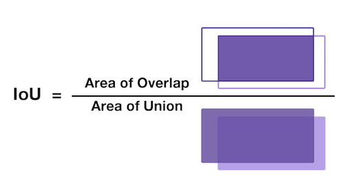
What is IOU ? IOU means Intersection over union. It is a measure that gives how much area you have in common between prediction and ground truth. Higher the IOU, better the prediction. So out of 5 predicted boxes, Yolo will choose the box with highest IOU. Below image helps to understand IOU better.

Collision : Let us say one cell itself is having multiple object. Let us take the fig-2 and assume that bottle & laptop are in same cell. Yolo predicts 5 bounding boxes per cell. Let us see how bounding boxes are getting assigned to bottle & laptop in this case. Yolo uses a method called collision in such instances. This is how it happens.

• Yolo predicts the classes for the objects identified in the cell and objectness score.
• Yolo predicts the centroid & bb scale coordinates for the classes.
• Yolo calculates the area of scaled bounding boxes for each of the anchor boxes.
• Then it calculates IOU corresponding to each bounding box for each object.
• Anchor box that gets the best IOU will be selected & BB created out of that anchor box will be used forward.
• Let us name the 5 anchor boxes as A, B, C, D, E.
• Bottle is considered first. Anchors A, B, C, D, E share an IOU of 0.73, 0.57, 0.61, 0.52 and 0.45 respectively for bottle. Hence anchor A is assigned as it has highest IOU 0.73
• Next laptop is considered. Imagine laptop shares an IOU of 0.74, 0.68, 0.59, 0.53 and 0.47 with anchors A, B, C, D and E respectively.
• Now Yolo recognizes that laptop is better match for anchor A.
• Accordingly, it reassigns anchor A to laptop and assign Anchor C – the next best match (0.61) – to bottle.

8. How to decide the number of anchor boxes to be used ?

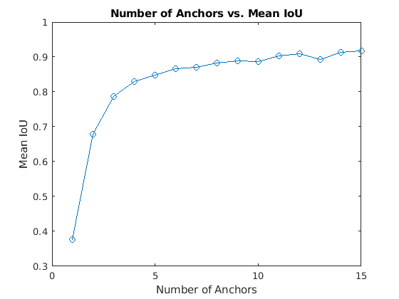
Anchor boxes are critical in determining the bounding boxes and thereby for Yolo object detection. So are we choosing the number of anchor boxes randomly ? No ! As part of pre-processing, we will pass the training data through a K-Means clustering and will choose a number that gives an optimal result between IOU and performance. Let us say we have 1 million unique objects in our dataset. We will get a mean IOU (Total IOU / No: of Images) of 1 if we choose 1 million BB. But this is not practical. Also beyond a certain point, IOU curve will flatten i.e. diminishing returns will start setting similar to what is shown below.
Hence Yolo researchers decided to settle on a number where algorithm can achieve good IOU without compromising performance (i.e. ability to detect on a real time basis). They tested Yolo on COCO and Imagenet datasets. Accordingly for Yolo V2 – 5 anchor boxes were used and in Yolo V5 – brought it down to 3 anchor boxes.

9. Yolo predictions

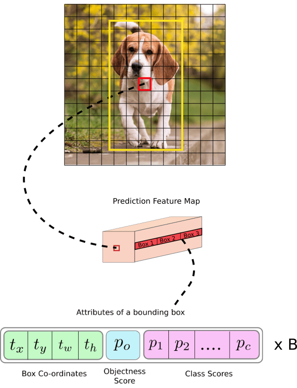
Based on what we understood so far, Yolo will predict class, objectness, centroid of object detected and bounding box scales. Let us try to visualize it.

• Image is broken down to S x S grid. In the above figure 13 x 13 cells.
• What we are seeing above with green steps is 1 such cell out of 169 cells.
• This cell will be having 5 anchor boxes (steps in figure).
• We are seeing expanded version on 1 such anchor box out of 5 anchor boxes.
• 1 anchor box will bound only 1 object. This anchor box will hold the objectness score of the object it detected (brown cell).
• Let us say we have 20 classes in our dataset. Prediction vector for the anchor box will have probability scores for these 20 classes (pink cells).
• Out of these 20, one that has highest score is the object that this specific anchor box detected (not shown in image).
• There will be 4 coordinates (yellow cells). First 2 coordinates belong to the centroid of the object detected.
• Next 2 coordinates belong to the bounding boxes (scaling factor).

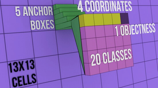
In the above image, each cell can have 5 anchor boxes, hence each cell can predict 5 different objects. Here, Yolo can predict a total of 169 * 5 = 845 objects out of entire 13×13 image grid . Each cell can have 5 anchor boxes each having 4 coordinates + 1 OS + 20 classes = 25 parameters. Hence one cell will hold 5 anchor boxes * 25 parameters = 125 predicted parameters. Below image will help to cement the concept further.

10. More on predictions

In Yolo, predictions are done using a fully convolutional network. We will get output in the form of a feature map in Yolo. As seen in previous section, each cell in this feature map can predict an object through one of its 5 bounding boxes provided center of the object falls in the receptive field of that cell (refer Fig-9). We mentioned in section 5 that Yolo will divide the input image of 416×416 to a 13×13 grid. Why divide to a grid and why 13×13 ? This to make sure that each cell-bounding box combination is responsible for detecting only 1 object. For this to happen, grid size (SxS) should be exactly matching to the output feature map size of Yolo. Hence, size of grid SxS will depend on (a) Network stride (b) Input image Size. Stride means factor by which a network down-samples the input image. If we are using a network with stride of 32 for an input image of 416×416, then final feature map size will be 416/32 = 13×13. So if Yolo uses such a network, then it should also divide the input image accordingly i.e. 13×13.

Let us examine below image to understand stride and structure of predictions better. Below stride is 32 and input image size is (608, 608, 3). Let us say we are dealing with Coco dataset that has 80 classes and are using a batch size of ‘m’. Then
(m, 608, 608, 3) -> CNN -> (m, 19, 19, 5, 85)
where 19, 19 is output feature map size (608/32 = 19), 5 is number of anchor boxes, and 85 = 80 classes + 5 bounding box coordinates

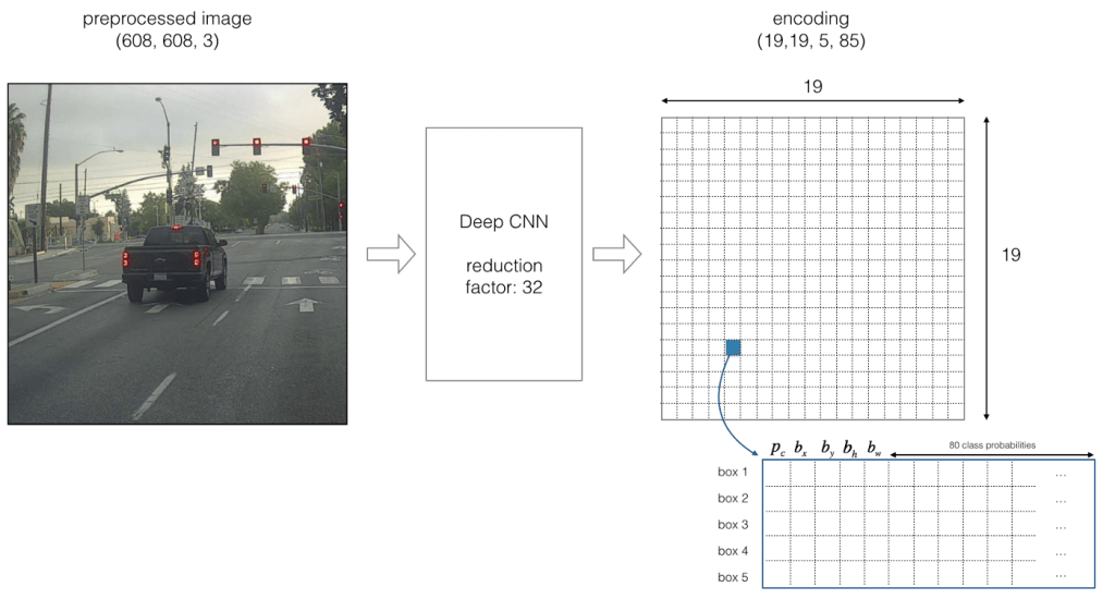
If center of an object falls on a particular cell (shown as blue in Fig-10), that cell is responsible for detecting that object. As we are using 5 anchor boxes, each of the 19×19 cells will carry information about 5 boxes. Structure of prediction vector for this will be as below.

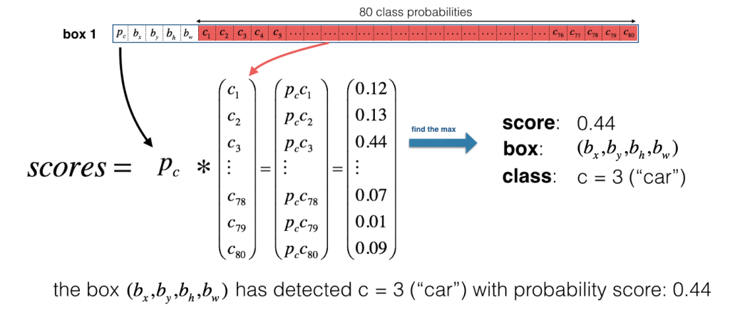
Now for each box (for each cell), predicted objectness score (Pc) is multiplied with class probabilities and max probability that comes out will be taken as the class of object detected. Refer below image.

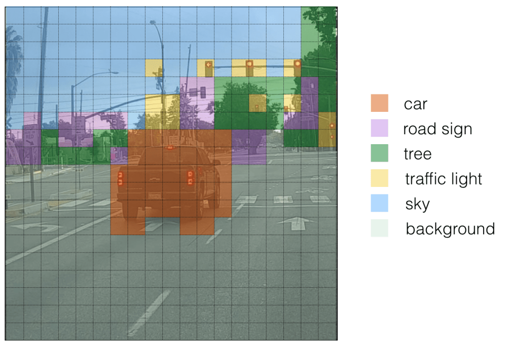
For ease of visualization let us assign different colours for each of the classes detected. Please note that this is not the output of Yolo but we can consider it as an intermediate state before non-maximum suppression (NMS).

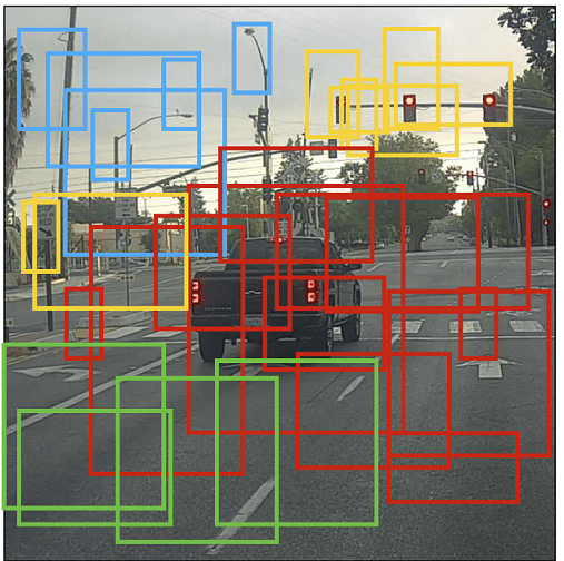
If we put bounding boxes around these objects, image will be as below. There are too many bounding boxes here but Yolo will bring down to 1 bounding box per object by using Non-Maximum Suppression (NMS).

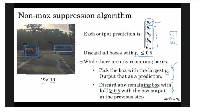
NMS : Below image shows how non-maximum suppression works & eliminates duplicate bounding boxes. Also refer the video link listed in source below to get a better intuition. Please note that Pc and IoU numbers given in below image are representative.

11. Center coordinates and Bounding Box coordinates

Why should Yolo predict scale by which anchor boxes need to be modified ? Why can’t it directly predict width and height of bounding boxes ? Answer – it is not pragmatic as it will cause unstable gradients while training. Instead, most modern object detectors including Yolo predicts log-space transforms or in other words – offsets and apply them to pre-defined anchor boxes. We already seen that Yolo predicts 4 coordinates around which bounding boxes are built. Following formula shows how bounding box dimensions are calculated from these predictions.

bx, by -> x, y center coordinates
bw,bh -> Width and height of bounding boxes
tx, ty, tw, th -> Yolo predictions (4 coordinates)
cx, cy -> Top-left coordinate of grid cell where object was located
Pw, Ph -> Anchor box width and heigth

Center Coordinates : Let us refer Fig-9. Dog is detected on (7,7) grid. When Yolo is predicting center coordinates (tx, ty), it is not predicting the absolute coordinates but offsets relative to the top-left coordinate of grid cell where object was located. Also these predictions will be normalized based on the cell dimensions from feature map. So for our dog image, if we get offset predictions as (0.6, 0.4) then in feature map it will be (6.6, 6.4). What if offsets predicted are 1.6 & 1.4 ? Coordinates will now be (7.6,7.4) taking object to grid location (8,8). But this breaks the Yolo rule which says cell that detected object (7,7) itself should be responsible for it. Hence we will pass the center coordinate predictions via sigmoid forcing the values to stay between 0 and 1 thereby keeping the grid location at (7,7) itself. As we covered equations 1 & 2 that gives bx, by let us move on to discuss bounding box coordinates.

Dimensions of bounding box (bw, bh) are obtained by applying log-space transformation to the predicted output (tw, th) and then mutiplying these with anchor box dimensions (Pw, Ph). This explains equations 3 & 4 above. These dimensions are normalized based on image height & width. This means if we get (0.3, 0.4) as output, in a 13×13 feature map, actual width and height of bounding box will be (13*0.3, 13*0.4). Below image visualizes the 4 equations given in Fig-15.

12. Yolo Loss Functions

Now let us take a look at loss function to understand how network trains and improves in object detection.

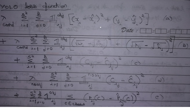
Yolo loss function is having 5 parts as shown in equation as a, b, c, d, e.

Let us start with (e) first. This part is dealing with classifying the object. This is same as the squared error loss functions used in image classification except the summations part and 1obj factor.

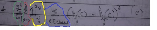
What we are doing via this equation is as follows. We are comparing the predicted class Pij(C)-Hat with ground truth Pij(C). We will do this for :

• Each cell in grid (green curve ) from 1 to 13^2, i.e for each of 169 cells. In our case S=13 hence 13^2.
• For each box inside each of the cells (red curve) i.e. 1 to B=5 as we are dealing with 5 anchor boxes
• For each class (Blue curve), if there are 80 classes then C = 80
• We will multiply each of the above occurrences with 1obj. This will help us to consider only those cells that is above a certain objectness threshold (section 5). More on this below.

Let us now examine (C). This part deals with cells that have object inside it.

• Summations and loop remains the same.
• Meaning of 1obj remains the same. Only those cells that are above the objectness threshold will get a value of 1obj as 1. Remaining all cells will have 1obj = 0 and will be ignored.
• For those cells with 1obj = 1, Cij (ground truth) will be assigned 1. This GT objectness score is compared with predicted objectness score Cij-hat
• Let us say in fig-9 only cell (7,7) met the threshold criteria and Yolo found that 3rd anchor has best IOU. Then only cell (7,7) i.e. i = 49 and anchor j=3 will have objectness score 1obj = 1.
• In other words i = 49, j= 3 instance of 1obj will be 1, all other occurrences 0.
• Let us say network predicted Cij-hat as 0.7 for this cell. Then loss value for this cell will be 1 * ( 1 – 0.7 )^2.

Next, let us see interpret (d). This part deals with cells having no-object inside it. It is equally important to assess & reduce false positives i.e. Yolo detecting an object when actually there is none. Part (d) serves this purpose.

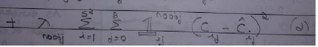
• Summations and loop remains the same as in previous sections.
• Instead of 1obj we have 1noobj here. We will call 1noobj as No-objectness number. Here those cells that are above the threshold, will be assigned 1noobj = 0. This is because these cells have an object inside them. Remaining all cells will have 1noobj = 1.
• For earlier example, only for cell (7,7) i.e. i = 49 and anchor j=3 will have no-objectness score 1noobj = 0.
• In other words i = 49, j= 3 instance of 1noobj will be 0, all other occurrences 1.
• Yolo introduced one more factor Lamda-noobj in the equation. This is to mitigate the effect of (d) compared to (c).
• For (c) only 1 cell (or few cells) will be having value whereas for (d) most of the cells will have a loss-value. Loss-function value for (c) will be much lesser compared to (d). In our example while (c) has value only for 1 cell, (d) has value for all 844 cells.
• Hence network will ignore (c) and focus on reducing (d). But we want both objectness and no-objectness predictions to improve.
• Hence, we will reduce the effect of no-objectness (d) by introducing Lamda-noobj.
• We will give a lesser value of Lamda-noobj (0.0001) at beginning to make the value comparable with (c). As trainining proceeds, we will keep slightly increasing Lamba-noobj to ensure that it remains on par with (c).
• Let us say for cell, i = 56, j =2 network predicted Cij-hat = 0.3.
• We know that there is no object in this cell so Cij = 0
• Through (d), Yolo built a way to punish this and value of loss function will be 0.0001 * 1 * (0 – 0.3)^2
  where 1noobj = 1, Lamda-noobj = 0.0001, Cij = 0 (no-object in this cell)

Finally, let us see what (a) and (b) are meant for.

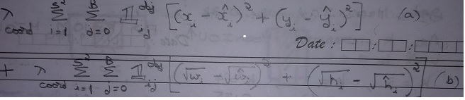
• This part deals with network learning about center location and bounding box dimensions.
• (a) deals with center location. xi and yi are ground truth coordinates supplied via training labels.
• xi-hat and yi-hat are network predictions that are compared with ground truth.
• (b) deals with bounding box width and height. wi and hi are ground truth dimensions supplied via training labels.
• wi-hat and hi-hat are network predictions that are compared with ground truth.
• We are using square root here to ensure that smaller bounding boxes are also optimized. Taking square root will magnify smaller errors & make them accountable.
  eg: Error = 0.0009 & Error ^ 0.5 = 0.03. If network encounters both these numbers, then it will prefer 0.03 over 0.0009 because 0.03 > 0.0009.
• There is a multiplication factor lamda-coord involved in both (a) and (b). In section 4, we mentioned “Initial epochs of Yolo network are trained only for classification.” lamda-coord is meant for this purpose.
• For initial epochs let us say 100 epochs, we will train only for classification and objectness. We achieve this by keeping lamda-coord = 0.
• In later epochs, we will train detection also by giving values to lamda-coord.

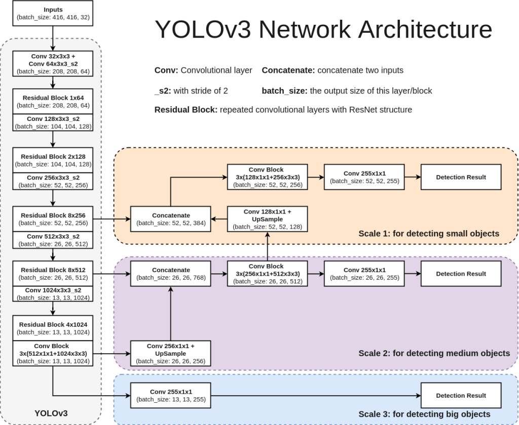
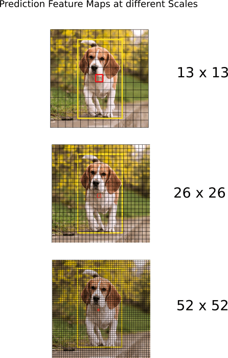
13. Network

Each version of Yolo comes with its own modification in CNN network. For sake of understanding, we will refer Yolo V3 network here. Network used for Yolo V3 is Darknet-53. It uses only convolutional layers. Instead of max-pooling it uses 3×3 with a stride of 2. Also, network predicts at 3 feature map scales – 13×13, 26×26, 52×52. Lower feature map scales were introduced to detect lower resolution objects. Below architecture diagram is self-explanatory to understand the network. Also shown below is how feature map predictions at 3 scales will look like.
Standard metric used for evaluation of Yolo network is mAP – Mean Average Precision. You can refer below two articles to get a better understanding on mAP.
Medium_JonathanHui_map
tarangshah_map

14. Conclusion

That’s it for Yolo intuition. Yolo is rapidly evolving. At the time of writing this article Yolo V5 is already out and we can expect more versions to be released in future. I would recommend reading those papers and understand what is different from previous versions. Hope you were able to understand how Yolo works now and reading this article enable you understand future revisions.