In this article, we will discuss those components of Convolutional neural network (CNN) where prediction of images and feedback for those predictions happen. First, let us take a bird’s eye view on how CNNs work:
1) Input images in the form of tensors will be fed to CNN.
2) Convolution layers will extract features.
3) At the final layer, network will classify the object using the features extracted.
4) Back propagation will provide feedback to the network comparing predictions VS ground truth.
5) Network will update the weights of kernels based on the feedback.
6) Steps 1 to 5 will repeat till we train our network (epochs).
Activation Functions and why they are needed ?
Activation Functions are used in CNNs on step 2 mentioned above. Let us find out why they are needed and how it helps CNN ?
Convolutions are sum-products of tensors as shown below. This is essentially a linear operation that can be expressed in the form of w0*x0 + w1*x1 + ….

But real-life problems are non-linear. For example, if a car is about to hit us, we will instantaneously jump to safety. If we plot the speed of car VS response, the curve will be non-linear.
Hence for CNNs to deal with complex problems, sum-of-products(linear results) that convolutions provide are not enough. We apply activation functions on our convolution outputs to deal with this. Activation functions bring non-linearity to the convolution output. Below is a pictorial representation of the same. Output of activation function is fed to the next convolution layer.

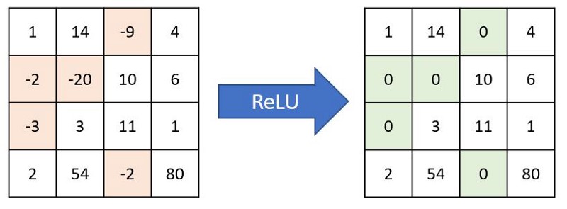
Most commonly used activation function is Relu (Rectified Linear Unit). Relu converts negative numbers to zeros and carry forward positive numbers. If a feature is not helping the network, then Relu won’t carry it forward (makes it zero), else carries it forward as such. Even though there are other activation functions like Sigmoid or tanh, Relu is preferred in most networks because of its simplicity and efficiency. Below is how Relu acts on a channel and gives back output.
Global Average Pooling (GAP)
To understand GAP concept, let us imagine a convolution layer trying to predict 10 different animals (10 classes). Below points should be kept in mind while we proceed.
a) For network to be effective, we should convolve till Receptive Field (RF) reaches >= image size.
b) Nodes in the final layer must be exactly same as number of classes we want to predict.
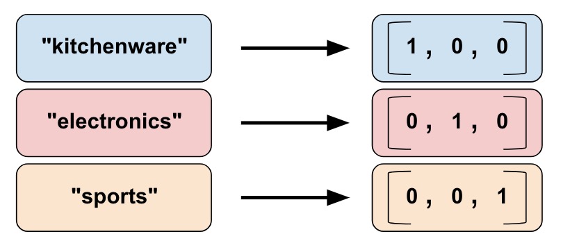
In this case, final layer passed to softmax for prediction needs to be 1x1x10. This 1x1x10 tensor is called one-hot vector because only one of the nodes (predicted class) will have value. An example for one-hot vector encoding is as below.
Lets us design convolution layers for our problem as below:
Layer 1 : 28 x 28 x 3 * 3 x 3 x 3 x 16, padding = True -> 28 x 28 x 16 (RF = 3)
Layer 2 : 28 x 28 x 16 * 3 x 3 x 16 x 32, padding = True -> 28 x 28 x 32 (RF = 5)
Layer 3 : 28 x 28 x 32 * Maxpooling -> 14 x 14 x 32 (RF =6)
Layer 4 : 14 x 14 x 32 * 3 x 3 x 32 x 32, padding = True -> 14 x 14 x 32 (RF=10)
Layer 5 : 14 x 14 x 32 * 3 x 3 x 32 x 32, padding = True -> 14 x 14 x32 (RF=14)
Layer 6 : 14 x 14 x 32 * Maxpooling -> 7x7x32 (RF = 16)
Layer 7 : 7 x 7 x 32 * 7 x 7 x 32 x 10 -> 1x1x10 (RF = 28)
Layer 8 : 1 x 1 x 10 * Softmax -> Predicted Output
Lets us focus on layer 7. This layer prepares data for final predictions. Here number of parameters involved will be 15,680 (7*7*32*10). This layer alone will make our model compute heavy.
In addition, by following this approach we have one more disadvantage. In layer 7, we are combining 32 channels to 10 channels. Ideally we can do this through 32*10 = 320 combinations. However by keeping prediction layer (layer 8) directly after layer 7, we are forcing 7x7x32 to act as a one-hot vector. This will cause 32 channels to be re-purposed solely for prediction purpose. Due to this, the combination is reduced from 32*10 to 32*1 limiting the ability to use features from 7x7x32 layer effectively. This scenario is shown in left part of below image.
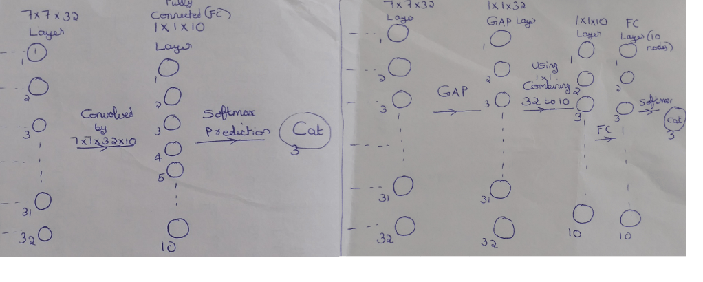
Now focus on the set-up shown in the right part of image.
– We are doing Global Average Pooling (GAP) to convert 7x7x32 to 1x1x32. We are taking average of 49 values to reduce it to 1 value per channel. (Since parameters are not optimized, No: of model parameters = 0)
– Next we are combining the GAP output 1x1x32 using 1x1x32x10 to give 1x1x10. (No: of model parameters = 32*10 = 320)
– 1x1x10 is then connected to Fully Connected (FC) layer which is passed for Softmax prediction.
This approach takes out the pressure of one-hot encoding from 7 x 7 x 32 layer and enables the network to utilize layer 7 much better. Also, we have significantly reduced the model parameters with this approach. Below is an image showing GAP -> FC -> Softmax for prediction of 3 classes. Here GAP is converting 6x6x3 to 1x1x3.
Softmax
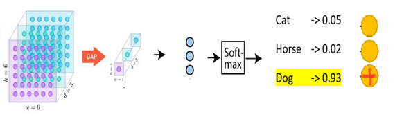
Softmax is a widely used activation function in CNN for image classification of single objects. Output of FC layer that we discussed above will be fed to Softmax. Below image shows where Softmax fits in a CNN architecture.
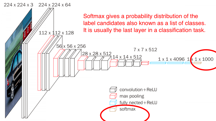
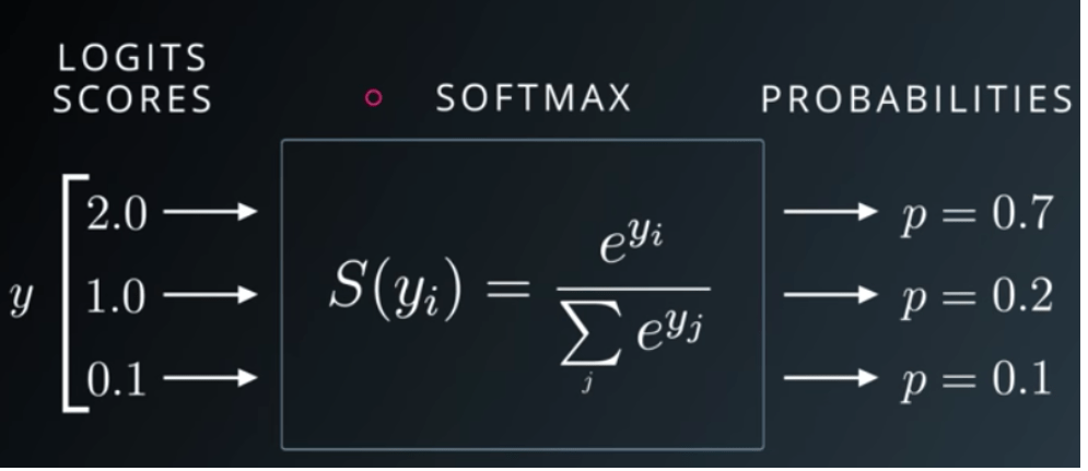
As seen above, Softmax is the final layer in CNN architecture and gives the probability distribution of list of classes. The class with the highest probability will be selected as the predicted class. The output of the softmax gives us the likelihood of a particular image belonging to a certain class. Formula for Softmax and how it helps predicting images is depicted in below snippets.
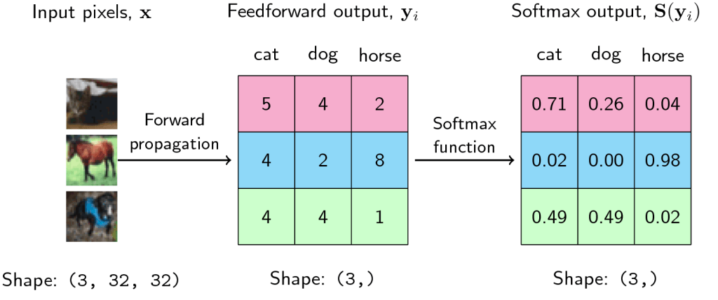
- In above image, each row shows probability of input image belonging to each of the 3 classes. Network predicts that it is a cat with 0.71 likelihood for first image.
- For second image, likelihood of the image being a horse is very high (0.98).
Let us inspect third scenario. Here likelihood of image being dog is same as that of cat (0.49). In reality these 2 numbers can never be same. Hence, it will be like probability of dog = 0.49001 and cat = 0.48999 or vice versa. Model will predict the class with higher probability. If model predicted that image is a dog, then prediction accuracy for this image is 100%. If it predicted cat, then accuracy drops to 0%. Margin between switching accuracy from 100% to 0% is very thin – 0.00002. Hence measuring accuracy alone can’t tell us how good our model is. We should be able to quantify how confident our model is about the class it predicted being true. This brings us to the concept of Negative Likelihood Loss.
What is Negative Likelihood Loss (NLL) and why is it required ?
We already seen that accuracy alone is insufficient to understand how good a model is. This becomes particularly important when predictions are made on the basis of a narrow margin. Let us take another example to further understand this concept.
Imagine there are 100 individuals in your village. An election is called upon to nominate the village head. Each of these 100 individuals stood as candidates for election. Incidentally 2 among them happens to be you and your spouse. Now all the remaining 98 individuals voted for themselves. You convinced your spouse to vote for you. When results are out, you won the elections. But the vote percentage you received is 2% compared to 1% for 98 others and 0% for your spouse. Here the result alone is not giving us accurate picture on how badly you won the elections.
This could happen in our CNN models also as seen in the dog vs cat example above. NLL gives us a measure on how confident a model is about predicting a class and hence throwing it out. It indicates the degree of confidence of model.
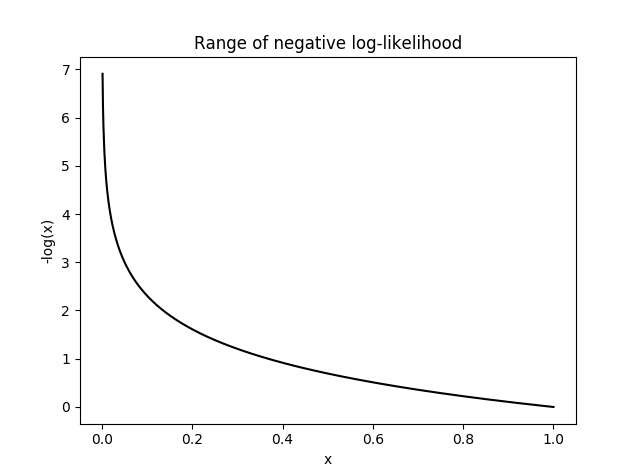
Formula for NLL is L(y) = -log(y) where y is prediction and L(y) is NLL.
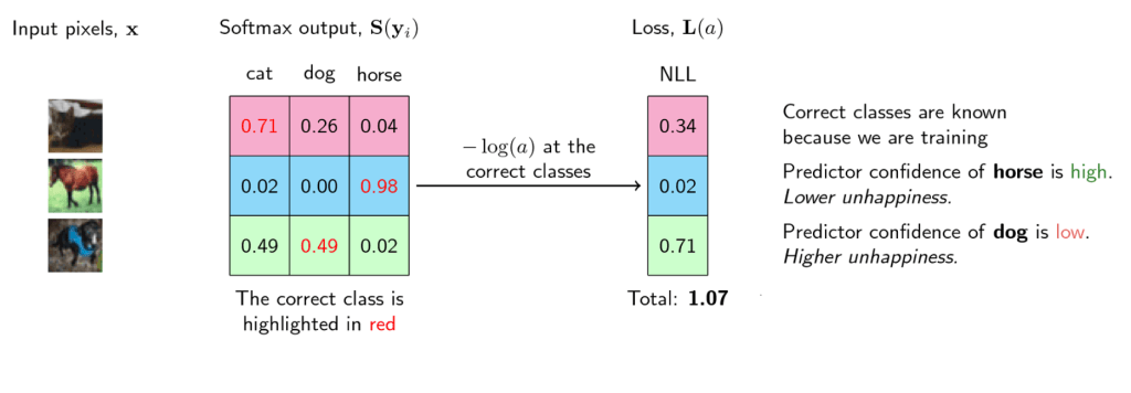
Below is the softmax table modified after adding NLL values. As we can see, lower the NLL value, happier the model (degree of confidence : high).
Graph for NLL is as follows. NLL becomes unhappy at smaller values, indicating that model is not predicting with enough confidence. It will become very sad (infinite unhappiness) when model confidence touches even smaller values. NLL becomes happy at larger x values indicating that model is predicting emphatically. What happens here is that in loss function, we will sum the losses of all the correct classes. So whenever the network assigns high confidence (x) for the correct class, the unhappiness (-log(x)) becomes low, and vice-versa.
Hope this article gave you an intuition on how final layers of a CNN operates and gives predictions.
