In Deep Neural Networks, maintaining same image size throughout the network is not sustainable due to huge computing resource it commands. At the same time, we also need enough convolutions to extract meaningful features. We learnt in last article that we can strike a balance between these two by down-sizing at proper intervals. In this article, we will discuss on how down-sizing is done. We will also cover how to combine channels using 1×1 convolutions and discuss Receptive Field (RF) calculation.
Why we need Max-Pooling ?
3×3 convolutions with a stride of 1 increase RF by 2 (details on stride here). Also, for effective image classification, RF should be >= size of image. Let us take an image of size 399×399 and imagine we only have 3×3 convolutions at our disposal. How many convolution layers will it take to reach RF of 399 ? Approximately 200 layers as shown below. Such a network will require huge computing power for processing.
399 * 3×3 -> 397 ; RF = 3
397 * 3×3 -> 395 ; RF = 5
395 * 3×3 -> 393 ; RF = 7
393 * 3×3 -> 391 ; RF = 9
391 * 3×3 -> 389 ; RF = 11
.
.
5 * 3X3 -> 3 ; RF = 397
3 * 3X3 -> 1 ; RF = 399
Hence, we need max-pooling to down-size the channel size at proper intervals so that we can get the job done within manageable number of convolutional layers. Below is how it looks like with max-pooling. We are reaching RF >= 399 in 30 layers (we will cover RF formula later).
399 | 397 | 395 | 393 | 391 | 389 | MP (2×2)
194 | 192 | 190 | 188 | 186 | 184 | MP (2×2)
92 | 90 | 88 | 86 | 84 | 82 | MP (2×2)
41 | 39 | 37 | 35 | 33 | 31 | MP (2×2)
15 | 13 | 11| 9 | 7 | 5 | 3 | 1
What is Max-Pooling ?
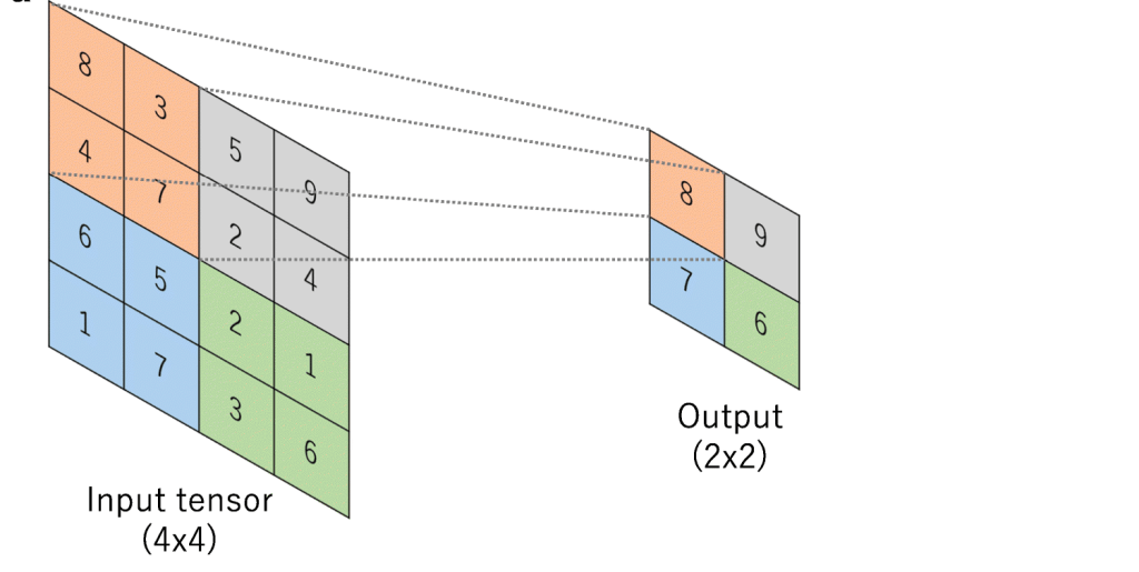
Max-Pooling is a convolution operation where kernel extracts the maximum value out of area that it convolves. Below image shows Max-pooling on a 4×4 channel using 2×2 kernel and stride of 2.
How to do Max-Pooling ?
Common practice is to use 2×2 kernel with a stride of 2. However kernels of any size can be used. We will get a single value out of the area covered. Hence bigger the size of kernel, higher the number of pixels getting omitted. Let us look at below scenario:
2×2 -> 1 out of 4 values selected
3×3 -> 1 out of 9 values selected
5×5 -> 1 out of 25 values selected
Bigger the kernel size, faster the compression. This may not be prudent. Hence most of the networks prefer 2×2 Max-Pooling with a stride of 2. Just to give you an intuition of how extraction happens, below is the image of 3×3 Max-Pooling with a stride of 3 .
When to use Max-Pooling ?
Rapid down-sizing is not sensible. It will lead to downsizing without extracting anything meaningful. Hence we should Max-Pool only at proper intervals. These intervals will vary based on the complexity of input images.
For example, in case of simple images like hand-written digits, we can Max-Pool at an interval of 5 RF i.e. 3×3 -> 3×3 -> Max-Pool. Whereas for complex problems like emotion detection we have to Max-Pool at higher RF intervals like 11 or more.
3×3 -> 3×3 -> 3×3 -> 3×3 -> 3×3 -> MP
This is because for hand-written digits even at an RF of 5, network should be able to extract meaningful features. But in problems like human emotion detection, input image is more complex and hence network has to convolve more to extract meaningful features. In this case, if we apply Max-Pool at RF =5, we will start down-size even before any meaningful extraction. It will be akin to downsizing a product team before development completion.
By omitting pixel values are we reducing our opportunity to learn more ? As discussed in earlier point, we start Max-Pooling only once we get a confidence that meaningful features are already extracted. By following this approach, we will be able to retain the relevant features and make them available for future layers to learn.
Retaining all the pixel values may help network to learn more but is it really required ? In most cases, no. If we can accurately detect an object with lesser parameters, we should go for it rather than over-learning and waste resources.
In addition to the above point, removing irrelevant features are equally important. eg: background in a dog image need not be carried forward. Through Max-Pooling we are accomplishing this objective too.
Why we take maximum value ? This is to ensure that most prominent feature is carried forward for future layers of network to learn. In CNN convention, bigger the channel value more important the feature. Through back-propagation, network will ensure that prominent features are getting higher values.
Eg: If the door knob of a house is important in an image classification problem, then irrespective of size of door knob compared to overall image, network will ensure that it gets carried forward till final layer. Network does this by assigning higher values to associated features.
What if all the values are similar ? Makes our life easier. This means, all the features in those channels are similar and we are just picking most relevant out of these similar features.
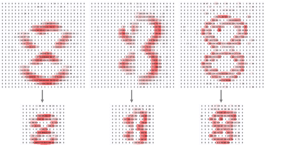
Below image shows how Max-pooling works in digit recognition problem. We can see that bigger pixel values are carried forward without losing any spatial information (8 still looks 8).
1 x 1 convolutions
In CNNs, we generally extract features using 3×3 convolutions. We store these features in separate channels like vertical edge in one channel, 135 degree edge in another etc.
While convolving, the approach we use is as follows – start with smaller number of channels and then increase number of channels. Rational is to start with simple features like edges and gradients which will be stored in lesser number of channels. Then we will build complex things like patterns, textures, part of objects etc. out of these simple features. We will store these complex features in variety of ways using higher number of channels.
Let us try to understand how 1×1 convolutions helps our above approach, by examining Squeeze-expand (SE) architecture. Please note that use of 1×1 convolutions is not limited to SE. We are just using SE here to understand the concept. Squeeze expand architecture increases number of channels step-by-step each block. When next block starts, we again start with smaller number of channels and keep increasing channels step-by-step.
Below is an example of squeeze expand network:
We will be focusing our discussion on the highlighted operation. Before we start, please keep below two points in mind. For more details on these, refer here.
a) No: of channels in kernels need to be same as number of channels in input
b) No: of kernels we want to convolve depends on number of channels we want in output.
Let us understand what is happening above:
392x392x256 | (3x3x256)x512 | 390x390x512 RF of 11X11
CONVOLUTION BLOCK 1 ENDS
TRANSITION BLOCK 1 BEGINS
MAXPOOLING(2×2)
195x195x512 | (1x1x512)x32 | 195x195x32 RF of 22×22
TRANSITION BLOCK 1 ENDS
First convolution
392x392x256 | (3x3x256)x512 | 390x390x512 RF of 11X11
Here 256 channels of 392×392 size are convolved by 512 kernels of size 3x3x256 to get 512 channels of 390×390 (No padding).
Second convolution
MAXPOOLING(2×2)
Max-Pooling using 2×2 kernel with stride 2 to get back 512 half-sized channels i.e. 512 channels of 195×195 size (half of 390×390).
Third convolution
195x195x512 | (1x1x512)x32 | 195x195x32 RF of 22×22
Here we are combining 512 channels of 195×195 size using 32 channels of size 1x1x512 to get back 32 channels of size 195×195.
Essentially the purpose of 1×1 convolution is to combine channels to give richer channels. What do richer channels mean ? Let us say we have 3 channels – one stores left eye, second stores right eye and third stores forehead. What 1×1 can do is combine all these 3 channels to give back a single channel that stores upper portion of human face.
1×1 retains height (H), width ![]() of channel while combining depth (D) to single pixel. Below is an example of single 1x1xD kernel convolving on D channels of size HxW to give back a single HxW channel. Here 1×1 is combining D channels to a single channel.
of channel while combining depth (D) to single pixel. Below is an example of single 1x1xD kernel convolving on D channels of size HxW to give back a single HxW channel. Here 1×1 is combining D channels to a single channel.
HxWxD | 1x1xDx1 | HxWx1
Why 1×1 has D channels (1x1xD) ?
Because input channel has D channels (HxWxD). No: of channels in kernels need to be same as number of channels in input.
Why we are using only 1 kernel (1x1x10x1) ?
Because we need only 1 channel in output for this particular case. No: of kernels we want to convolve depends on number of channels we want in output.
Let us look at one more example. Image below shows four 1x1x10 kernels convolving over 10 channels of 32×32 size to give back four channels of 32×32 size.
32x32x10 | 1x1x10x4 | 32x32x4
Here 1×1 is combining 10 channels to 4 channels.
Why 1×1 has 10 channels (1x1x10) ?
Because input channel has 10 channels (32x32x10). No: of channels in kernels need to be same as number of channels in input.
Why we are using 4 kernels (1x1x10x4) ?
Because we need 4 channels in output for this particular case. No: of kernels we want to convolve depends on number of channels we want in output.
1×1 calculations : Below image will give an idea on calculations that happen while using 1×1 convolutions.
– In first set, 6x6x1 is convolved by a single 1x1x1 kernel to give back 6x6x1. Please note that 1x1x1 kernel is a single value & in this example its value is 2.
– In second set, 6x6x32 is convolved by 1x1x32 kernel. Here # of kernels is kept open. 1x1x32 will be having 32 values across the depth. Each value in the 6×6 channel across the depth will be multiplied by its corresponding 1×1 kernel value and all these will be combined to give a single cell. This way we will get 6x6x(# kernels) in return. Please refer the image “1×1 convolution HxWxD | 1x1xD | HxWx1” if you want help visualizing this.
Another important advantage of 1×1 convolution is that it reduces burden of channel selection from 3×3.
Example : We want to predict dog, cat and tiger from a set of images. We gave image of tiger as input. In a particular layer we are at 28x28x256 channel size and want to get 16 channels out of this convolution. We only have 3×3 at our disposal. In this case, 16 different 3x3x256 kernels has to convolve to give 16 channels. Not all these 256 channels from input will be relevant for tiger. But 3×3 can figure this out only based on feedback it receives from back-propagation.
Suppose in this case, we are allowed to use 1×1. Then, we can combine our 256 channels to 16 channels using 1×1 convolution and pass only 16 channels for 3×3. In this case, only 16 different 3x3x16 has to convolve on 28x28x16 channel. We are significantly reducing number of parameters in the latter case.
This makes network faster as 3×3 can now decide relevant tiger channels from 16 instead of 256.
Receptive Field Calculation
Before we wrap-up this article, let us check the way in which we calculate the RF.
Below is the formula for the RF. Note that r -> RF , j -> jump
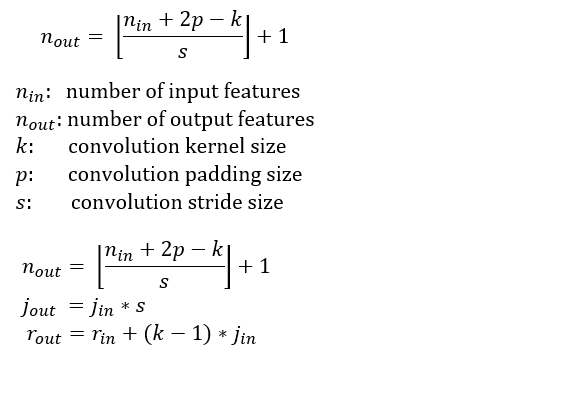
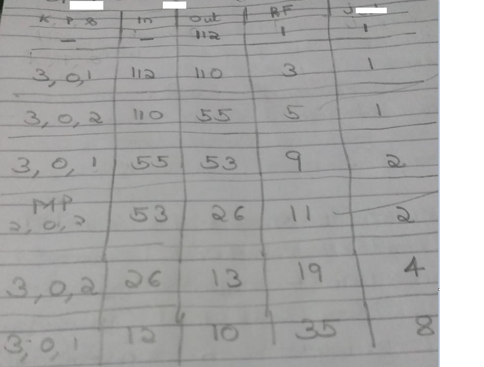
Attached below is a sample calculation so that we can understand how the formula works. Few points to note while going through below table. Write down Jump-out of layer 3, while doing calculations of layer 2 and so on.For Layer 1 : Jump-In = Jump-out = 1, Out = Input Size
For Layer 2 : Jump-In = Jump-out of layer 1
Jump-Out = Jump-In * stride
For Layer 3 : Jump-In = Jump-out of layer 2
Jump-Out = Jump-In * stride
………….
………….
For Layer 1 : RF-In = RF-out = 1
For Layer 2 : RF-In = RF-out of layer 1
RF-Out = RF-In * stride
For Layer 3 : RF-In = RF-out of layer 2
RF-Out = RF-In * stride
………….
………….