In last week article, we got a high level view on how neural networks identify objects. This week, we will cover items that will help us understand the concept of receptive field and why it is important in neural networks. You can find my last week article here.
What is receptive field (RF) ? Let us look into the below image.
For sake of understanding, imagine the animation above as a simple neural network. There are 3 layers in this network 5×5 -> 3×3 -> 1×1. Notice the dark shadowed box moving over the pixels. This operation is called convolution. The blue square grid is input image with size 5×5. Box with shadow that is moving over image is called kernel (in this case size 3×3). We can see that 5×5 convolved with 3×3 kernel gives us 3×3 output (yellow). Yellow 3×3 when convolved again with 3×3 kernel results in 1×1.
Receptive Field is a term used to indicate how many pixels, a particular pixel in a layer has seen in total – both directly and indirectly. There are two kinds of RF – local and global. Local RF refers to the size of kernel. Global RF is what we commonly refer to as RF.
Let us take a closer look to understand what this means.
Layer 1 (Blue) : Each of the 25 pixels know only about itself. GRF = 1
Layer 2 (Yellow) : Each of the pixel have seen 3×3 pixels from layer 1 and hence knows them. Notice how the darker shades over blue panel translates to a single cell in yellow panel. Here GRF = 3
Layer 3 (Green) : There is only 1 pixel. This pixel has directly seen 3×3 pixels from layer 2 and knows them. But each of these layer 2 pixels already have info about 3×3 pixels from layer 1. Hence layer 3 pixel has indirectly seen all the 5×5 pixels. Hence GRF = 5. Keep in mind that our original image size is 5×5.
Relevance of receptive field
Computer vision networks that we are discussing belong to supervised learning models. We will feed labelled images (training set) to the model and make the model learn. Then we will feed the model with test images. We know the labels for these test set but we won’t tell that to model. Instead, we will ask model to predict based on what it learnt. Based on prediction vs ground-truth, we determine the accuracy of model. In the training process, neural networks will check the label (dog, cat etc.) and learn the characteristics for a particular object. After training on enough variety images, model will acquire enough knowledge to classify a dog as dog. This model once it identifies the characteristics of dog in a given image will be able to classify image as dog correctly.
We help the network learn by breaking down images to tensors and then reconstructing again step by step as shown below. Detailed explanation is in my article.
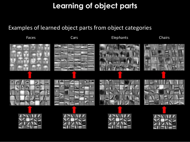
- We will break down image into basic channels.(We will cover channels later)
- The features inside these channels are then used to construct edges and gradients.
- Using these edges and gradients, we construct textures and patterns.
- From these textures and patterns, we build parts of objects.
- These parts of objects will be used to build objects.
In the above process of reconstruction, we are gradually increasing the RF of our network layer-by-layer. One point to note is that final layer RF must be = or > than size of original image. Let us understand this concept by answering few questions as below.
Why we need RF in final layer > or = to size of image ?
As we have seen, each pixel in a particular layer sees the world via pixels of its preceding layer. If you remember, final layer feeds the data to Softmax layer for classifying the object. Hence in order to share relevant data for classification, pixels in final layer must have seen the whole image. Imagine being tied to your seat in a theater and neck locked with blinders in such a way that you can see only in a straight line. Then you are asked to explain what is happening in movie. Obviously you wont be able to comprehend much visually. Same case applies to our final layer as well. We shouldn’t expect our network to predict a cat by only seeing let us say its tail or legs. This is the reason why we keep RF of final layer > or = to size of image. This way whole image gets captured in terms of RF in final layer.
Won’t reduction of size i.e. 5×5 -> 3×3 -> 1×1 be a problem ?
While increasing the RF, we reduce the size but still retains vital information. We are filtering useful information and keeping them in different channels. Imagine a box with 10 different masalas. We can combine them to make let us say 1000 different dishes. Here we started with 10 channels and went on to create 1000 unique channels. Similarly we are breaking down original image to edges & gradients (masalas) and then combine them to create more complex channels (dishes) at later layers. These complex channels eventually help us in classifying the objects via softmax.
Disclaimer : We will maintain the size same in each block via padding. But we will cover blocks and padding as we advance in future.
What is preventing us from maintaining original size throughout ?
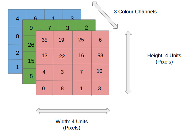
Snippet below shows 3 channels (RGB) each of size 4×4. Number of parameters involved = 4x4x3 = 48
At each layer, we can define as many channels as needed for network to gain better accuracy (32, 64, 128, 256 etc). Imagine 400×400 matrix maintained for 1024 channels in a single layer. This single layer alone will need 163 million parameters. DNNs can have more than 100 layers in certain networks. Hence maintaining same image size throughout the network won’t be sustainable because of huge computing power it demands. Also as discussed above, it is not required to get our job done.
Before we wrap-up this article, let us answer one more question . What is the role of convolutions here ? Convolutions help us perform the operations we mentioned above – increasing the RF as well as creating various channels. I will be covering convolutions in upcoming articles.
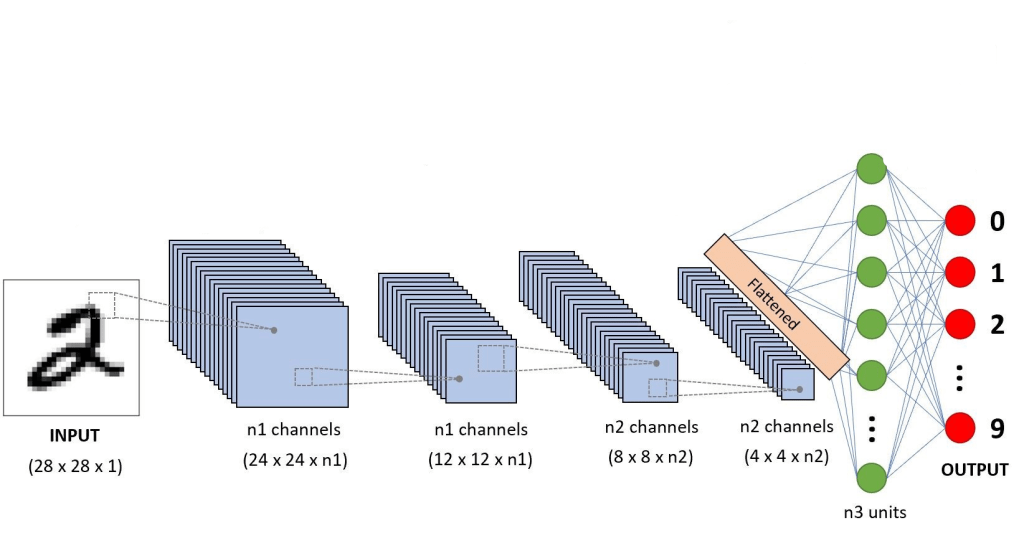
Below is a neural network where you can see number of channels increasing layer-by-layer and you can see why maintaining high channel size is not a good idea.